Interactive Rendering Trajectories Example
Copyright (c) 2014-2020 National Technology and Engineering Solutions of Sandia, LLC. Under the terms of Contract DE-NA0003525 with National Technology and Engineering Solutions of Sandia, LLC, the U.S. Government retains certain rights in this software.
Redistribution and use in source and binary forms, with or without modification, are permitted provided that the following conditions are met:
1. Redistributions of source code must retain the above copyright notice, this list of conditions and the following disclaimer.
2. Redistributions in binary form must reproduce the above copyright notice, this list of conditions and the following disclaimer in the documentation and/or other materials provided with the distribution.
THIS SOFTWARE IS PROVIDED BY THE COPYRIGHT HOLDERS AND CONTRIBUTORS “AS IS” AND ANY EXPRESS OR IMPLIED WARRANTIES, INCLUDING, BUT NOT LIMITED TO, THE IMPLIED WARRANTIES OF MERCHANTABILITY AND FITNESS FOR A PARTICULAR PURPOSE ARE DISCLAIMED. IN NO EVENT SHALL THE COPYRIGHT HOLDER OR CONTRIBUTORS BE LIABLE FOR ANY DIRECT, INDIRECT, INCIDENTAL, SPECIAL, EXEMPLARY, OR CONSEQUENTIAL DAMAGES (INCLUDING, BUT NOT LIMITED TO, PROCUREMENT OF SUBSTITUTE GOODS OR SERVICES; LOSS OF USE, DATA, OR PROFITS; OR BUSINESS INTERRUPTION) HOWEVER CAUSED AND ON ANY THEORY OF LIABILITY, WHETHER IN CONTRACT, STRICT LIABILITY, OR TORT (INCLUDING NEGLIGENCE OR OTHERWISE) ARISING IN ANY WAY OUT OF THE USE OF THIS SOFTWARE, EVEN IF ADVISED OF THE POSSIBILITY OF SUCH DAMAGE.
Tutorial showing many of the options available for rendering trajectories.
[1]:
from tracktable.domain.terrestrial import TrajectoryPointReader
from tracktable.analysis.assemble_trajectories import AssembleTrajectoryFromPoints
from tracktable.render.render_trajectories import render_trajectories, render_trajectories_separate
from tracktable.core import data_directory
import os.path
#Load sample data for rendering exmples
#Read in points and assemble trajectories
inFile = open(os.path.join(data_directory(), 'SampleFlightsUS.csv'))
reader = TrajectoryPointReader()
reader.input = inFile
reader.comment_character = '#'
reader.field_delimiter = ','
# Set columns for data we care about
reader.object_id_column = 0
reader.timestamp_column = 1
reader.coordinates[0] = 2
reader.coordinates[1] = 3
reader.set_real_field_column('altitude',4) #could be ints
reader.set_real_field_column('heading',5)
reader.set_real_field_column('speed',6)
builder = AssembleTrajectoryFromPoints()
builder.input = reader
builder.minimum_length = 3
trajs = list(builder.trajectories())
few_trajs = [traj for traj in trajs if traj[0].object_id == 'SSS019' or traj[0].object_id == 'TTT020']
INFO:tracktable.analysis.assemble_trajectoriesAssembleTrajectoryFromPoints:New trajectories will be declared after a separation of None distance units between two points or a time lapse of at least 0:30:00 (hours, minutes, seconds).
INFO:tracktable.analysis.assemble_trajectoriesAssembleTrajectoryFromPoints:Trajectories with fewer than 3 points will be discarded.
INFO:tracktable.analysis.assemble_trajectoriesAssembleTrajectoryFromPoints:Done assembling trajectories. 29 trajectories produced and 0 discarded for having fewer than 3 points.
[2]:
from tracktable.render.render_trajectories import render_trajectories
# The only required parameter is a list of trajectories. It's that simple.
render_trajectories(few_trajs)
# The default rendering assigns each object ID a hue which transitions from dark to light as the trajectory
# progresses. In addition, by default, a white dot shows the point with the latest timestamp in the trajectory.
# Hovering over a trajectory reveals its object_id, and clicking on a trajectory give the object_id and start and stop
# time for the entire trajectory
[2]:
[3]:
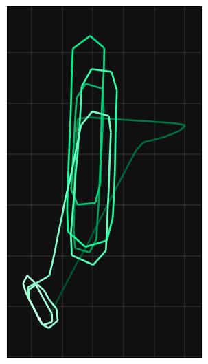
# Can use a different backend (default in Jupyter Notebooks is folium, default otherwise is cartopy)
# render_trajectories(few_trajs, backend='folium')
render_trajectories(few_trajs, backend='cartopy')
[3]:
<GeoAxesSubplot:>

[4]:
# Can render a single trajectory
render_trajectories(trajs[3])
[4]:
[5]:
# Can render a set of trajectories separately (each with their own map)
render_trajectories_separate(few_trajs)
[6]:
# You can change map tiles
render_trajectories(trajs[3], tiles='CartoDBPositron')
# Options include:
# OpenStreetMaps
# StamenTerrain
# StamenToner
# StamenWatercolor
# CartoDBPositron
# CartoDBDark_Matter
[6]:
[7]:
# You can specify a map tile server by URL # must include attribution(attr) string
render_trajectories(trajs[3], tiles='http://server.arcgisonline.com/ArcGIS/rest/services/NatGeo_World_Map/MapServer/tile/{z}/{y}/{x}', attr='ESRI')
[7]:
[8]:
# Can specify a bounding box (default extent shows all input trajectories)
# format of map_bbox is [minLon, minLat, maxLon, maxLat]
render_trajectories(few_trajs, map_bbox=[-108.081, 39.3078, -104.811, 41.27])
[8]:
[9]:
# Can specify specific object_ids to render as a string...
render_trajectories(trajs, obj_ids="VVV022")
[9]:
[10]:
# ... or a list of strings
render_trajectories(trajs, obj_ids=["JJJ010", "LLL012"])
[10]:
[11]:
# Can specify a solid color for all trajectories ...
render_trajectories([trajs[0], trajs[12]], line_color = 'red')
#Other color strings include: ‘red’, ‘blue’, ‘green’, ‘purple’, ‘orange’, ‘darkred’,’lightred’, ‘beige’,
#‘darkblue’, ‘darkgreen’, ‘cadetblue’, ‘darkpurple’, ‘white’, ‘pink’, ‘lightblue’, ‘lightgreen’, ‘gray’,
#‘black’, ‘lightgray’
[11]:
[12]:
# ... or a list of colors. Note you can use hex string notation for the colors as well.
render_trajectories([trajs[0], trajs[12]], line_color = ['red', '#0000FF'])
# Hex string notation is of the format #RRGGBBAA,
# Red Green Blue values from 0 to 255 as 2 hex digits each,
# and an OPTIONAL alpha (opacity) value with same range and format.
[12]:
[13]:
# The trajectories can be colored using a colormap ...
render_trajectories([trajs[0], trajs[12]], color_map = 'BrBG')
[13]:
[14]:
# ... or a list of color maps
render_trajectories([trajs[0], trajs[12]], color_map = ['BrBG', 'plasma'])
[14]:
[15]:
# You can even define your own color maps
import matplotlib.cm
import numpy as np
blues_map = matplotlib.cm.get_cmap('Blues', 256)
newcolors = blues_map(np.linspace(0, 1, 256))
pink = np.array([248/256, 24/256, 148/256, 1])
newcolors[:25, :] = pink # pink for takeoff (first ~10% of trajectory)
render_trajectories([trajs[0], trajs[12]], color_map = matplotlib.colors.ListedColormap(newcolors))
[15]:
[16]:
# You can specify a hue as a float between 0 and 1 which will be used to create a gradient that transitions form dark
# to light as the trajectory progresses
render_trajectories([trajs[0], trajs[12]], gradient_hue = .5)
[16]:
[17]:
# As with other color options, a list of hues can be used as well.
render_trajectories([trajs[0], trajs[12]], gradient_hue = [.25, .66])
[17]:
[18]:
# Hues can be derived from an rgb color specified as a color name or hex string color
render_trajectories([trajs[0], trajs[12]], gradient_hue = ['#00FF00', 'orange'])
[18]:
[19]:
#You can specify custom scalar mappings. In this case the color gets lighter as altitude increases.
import matplotlib.colors
def altitude_generator(trajectory):
#N-1 segments show altitude at beginning point
return [point.properties['altitude'] for point in trajectory[:-1]]
#Note: be sure to include the generator, and the scale for mapping scalars to the color map.
render_trajectories([trajs[16]], trajectory_scalar_generator = altitude_generator,
color_scale = matplotlib.colors.Normalize(vmin=0, vmax=35000))
[19]:
[20]:
#The linewidth of the trajectories can be adjusted. Default is 2.5 in folium
render_trajectories(trajs[26], linewidth=5)
[20]:
[21]:
# You can also adjust the width of the trajectory by some scalar. In this case the trajectory starts out very narrow
# and gets wider at each point it passes (as it progresses), but the color remains green throughout.
from tracktable.render.render_trajectories import progress_linewidth_generator
render_trajectories(trajs[28], line_color='green', trajectory_linewidth_generator=progress_linewidth_generator)
[21]:
[22]:
# You can also show the sample points along the trajectory. By default the points are colored consistent with line
# segments
render_trajectories(trajs[15], show_points=True)
# Hovering over a point gives the timestamp of that point and by default, clicking on a point reveals the object_id,
# timestamp, Latitude, and Longitude of that point.
[22]:
[23]:
# You can specify any set of properties to view when clicking on a point:
render_trajectories(trajs[15], show_points=True, point_popup_properties = ['altitude', 'heading', 'speed'])
# Clicking on a point now additionaly reveals the altitude, heading, and speed.
[23]:
[24]:
# The colors of all points can be specified
render_trajectories(trajs[15], point_color='red', show_points=True)
[24]:
[25]:
# The color and radius of the dot at the close of the trajectory can be changed
render_trajectories(trajs[24], dot_color='red', dot_size=5)
[25]:
[26]:
# To not show the dot at the close of the trajectory:
render_trajectories(trajs[24], show_dot=False)
[26]:
[27]:
# In folium the distance geometry calculations can be shown. Default depth is 4
render_trajectories(trajs[25], show_distance_geometry=True, distance_geometry_depth=4)
#red are level 1 lines
#blue are leve 2 lines
#yellow are level 3 lines
# and purple are level 4 lines
#hovering over the lines gives the normalized length of each line
[27]:
[28]:
# Save trajectories (as html file) to a default unique filename (trajs+datetimestamp+.html)
render_trajectories(trajs[20:22], save=True)
[28]:
[29]:
# Save trajectories (as html file) to a given filename/path and don't render to the notebook
# (; at end of line (or assigning output to a variable) causes map to not be rendered in the notebook)
render_trajectories(trajs[23], save=True, filename='tmp_my_tracks.html')
[29]:
[30]:
# If render_trajectories is not the last function in a cell the map won't render
render_trajectories(trajs[24])
print('A nice trajectory')
A nice trajectory
[31]:
# To overcome this, set show=True to force rendering to the notebook
render_trajectories(trajs[24], show=True)
print('A nice trajectory')
A nice trajectory
[32]:
# or, assign the returned map to a variable, and list the variable name alone on the last line of the cell
m=render_trajectories(trajs[24])
print('A nice trajectory')
m
A nice trajectory
[32]:
[33]:
# Can use cartopy as backend and save imgaes
render_trajectories(trajs[23], backend='cartopy', save=True, filename='tmp_my_tracks.png')
[33]:
<GeoAxesSubplot:>
[ ]: