Trajectory Clustering Example

Copyright (c) 2014-2020 National Technology and Engineering Solutions of Sandia, LLC. Under the terms of Contract DE-NA0003525 with National Technology and Engineering Solutions of Sandia, LLC, the U.S. Government retains certain rights in this software.

Redistribution and use in source and binary forms, with or without modification, are permitted provided that the following conditions are met:

1. Redistributions of source code must retain the above copyright notice, this list of conditions and the following disclaimer.

2. Redistributions in binary form must reproduce the above copyright notice, this list of conditions and the following disclaimer in the documentation and/or other materials provided with the distribution.

THIS SOFTWARE IS PROVIDED BY THE COPYRIGHT HOLDERS AND CONTRIBUTORS “AS IS” AND ANY EXPRESS OR IMPLIED WARRANTIES, INCLUDING, BUT NOT LIMITED TO, THE IMPLIED WARRANTIES OF MERCHANTABILITY AND FITNESS FOR A PARTICULAR PURPOSE ARE DISCLAIMED. IN NO EVENT SHALL THE COPYRIGHT HOLDER OR CONTRIBUTORS BE LIABLE FOR ANY DIRECT, INDIRECT, INCIDENTAL, SPECIAL, EXEMPLARY, OR CONSEQUENTIAL DAMAGES (INCLUDING, BUT NOT LIMITED TO, PROCUREMENT OF SUBSTITUTE GOODS OR SERVICES; LOSS OF USE, DATA, OR PROFITS; OR BUSINESS INTERRUPTION) HOWEVER CAUSED AND ON ANY THEORY OF LIABILITY, WHETHER IN CONTRACT, STRICT LIABILITY, OR TORT (INCLUDING NEGLIGENCE OR OTHERWISE) ARISING IN ANY WAY OUT OF THE USE OF THIS SOFTWARE, EVEN IF ADVISED OF THE POSSIBILITY OF SUCH DAMAGE.

This notebook is an end-to-end example of how to cluster trajectories in Tracktable using distance geometry. It goes through the following steps:

1. Read in points from a file.

2. Assemble those points into trajectories.

3. Create a distance geometry signature for each trajectory.

4. Using those signatures as feature vectors, compute clusters using DBSCAN.

5. Print statistics about each cluster.

6. Render the resulting clusters onto a map.

Eventually, distance geometry computation will move into the library itself.

# Set up Matplotlib to render in a notebook before anyone else can change its back end.
%matplotlib inline
import matplotlib

Matplotlib is building the font cache; this may take a moment.

Compute an N-point distance geometry signature

Distance geometry is a technique for characterizing a curve in space by measuring the distances between evenly spaced points (called control points) on the curve. This implementation has three parameters:

  1. A trajectory

  2. The number of control points

  3. Whether to normalize the distances in the signature so that the largest distance is always 1.

The number of control points controls the fidelity of the resulting signature. The more control points, the more accurately the features of the curve can be represented, but the longer it takes to compute.

Normalizing the distance allows shape-based comparison between trajectories by taking the dot product of their respective distance geometry signatures. The higher the dot product, the more similar the trajectories. There are many possible normalization schemes; this is the one we find useful.

Returns:

  tracktable.domain.feature_vectors.FeatureVectorNN where NN is the size of the resulting distance geometry signature.

from tracktable.domain.feature_vectors import convert_to_feature_vector
from tracktable.core.geomath import point_at_length_fraction
from tracktable.core.geomath import distance
from tracktable.core.geomath import length

from tracktable.analysis.distance_geometry import distance_geometry_by_distance

Now we are going to gather our points from file and assemble them into trajectories. We will use the same point reader and trajectory builder we used in previous examples. Then, we will compute the cluster labels.

from tracktable.domain.terrestrial import TrajectoryPointReader
from tracktable.analysis.assemble_trajectories import AssembleTrajectoryFromPoints
from tracktable.analysis.dbscan import compute_cluster_labels
from tracktable.core import data_directory
from datetime import timedelta
import cartopy
import cartopy.crs
import os.path

data_filename = os.path.join(data_directory(), 'SampleFlightsUS.csv')
inFile = open(data_filename, 'r')
reader = TrajectoryPointReader()
reader.input = inFile
reader.comment_character = '#'
reader.field_delimiter = ','
reader.object_id_column = 0
reader.timestamp_column = 1
reader.coordinates[0] = 2
reader.coordinates[1] = 3

builder = AssembleTrajectoryFromPoints()
builder.input = reader
builder.minimum_length = 5
builder.separation_time = timedelta(minutes=10)


all_trajectories = list(builder)
# Get feature vectors for each trajectory describing their distance geometry
depth = 4
feature_vectors = [distance_geometry_by_distance(trajectory, depth)
                   for trajectory in all_trajectories]

# DBSCAN needs two parameters
#  1. Size of the box that defines when two points are close enough to one another to
#     belong to the same cluster.
#  2. Minimum number of points in a cluster
#
signature_length = len(feature_vectors[0])

# This is the default search box size. Feel free to change to fit your data.
search_box_span = [0.06] * signature_length
minimum_cluster_size = 2

cluster_labels = compute_cluster_labels(feature_vectors, search_box_span, minimum_cluster_size)

INFO:tracktable.analysis.assemble_trajectoriesAssembleTrajectoryFromPoints:New trajectories will be declared after a separation of None distance units between two points or a time lapse of at least 0:10:00 (hours, minutes, seconds).
INFO:tracktable.analysis.assemble_trajectoriesAssembleTrajectoryFromPoints:Trajectories with fewer than 5 points will be discarded.
INFO:tracktable.analysis.assemble_trajectoriesAssembleTrajectoryFromPoints:Done assembling trajectories. 30 trajectories produced and 1 discarded for having fewer than 5 points.

Cluster Statistics

Here we calculate the size of the clusters we labeled.

# Assemble each cluster as a list of its component trajectories.
clusters = {}
for(vertex_id, cluster_id) in cluster_labels:
    if cluster_id not in clusters:
        clusters[cluster_id] = [all_trajectories[vertex_id]]
    else:
        clusters[cluster_id].append(all_trajectories[vertex_id])

# If a cluster does not have an id, it is an outlier
def cluster_name(cid):
    if cid == 0:
        return 'Outliers'
    else:
        return 'Cluster {}'.format(cid)

#Print the cluster id and the number of trajectories in the cluster.
print("RESULT: Cluster sizes:")
for(cid, cluster) in clusters.items():
    print("{}: {}".format(cluster_name(cid), len(cluster)))

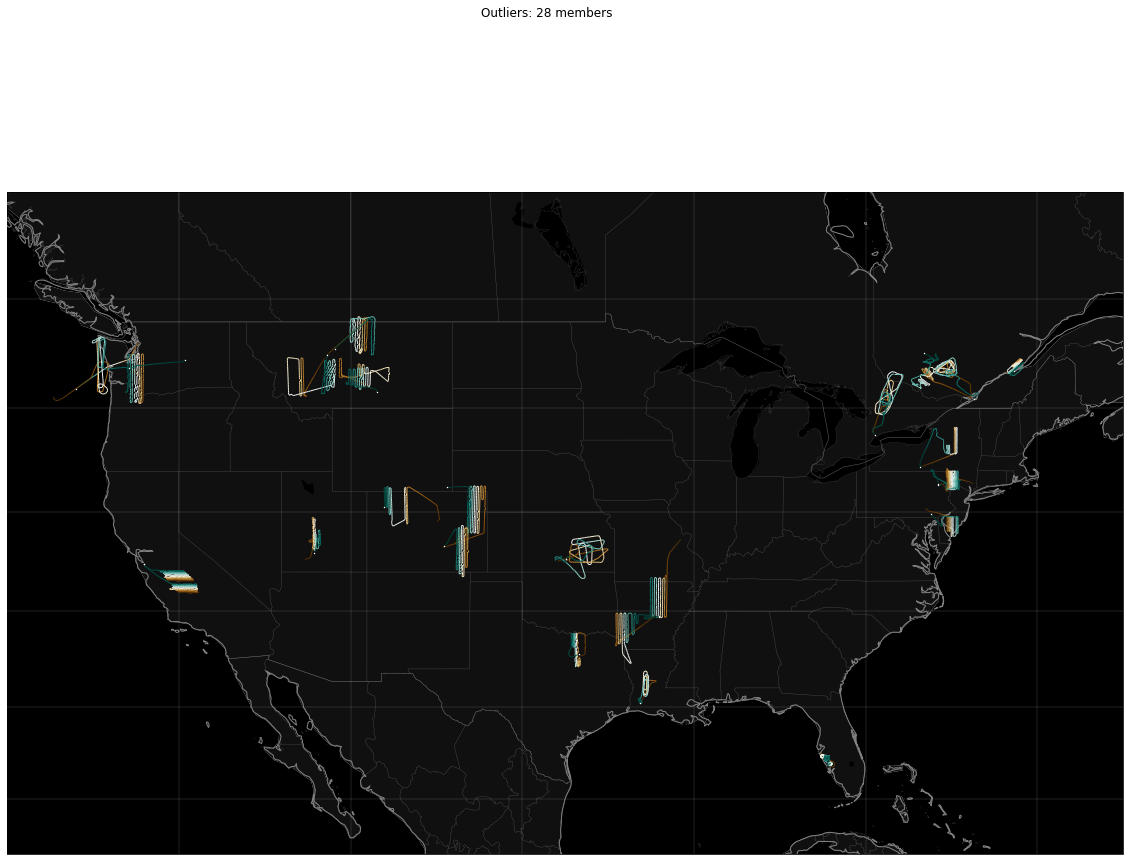
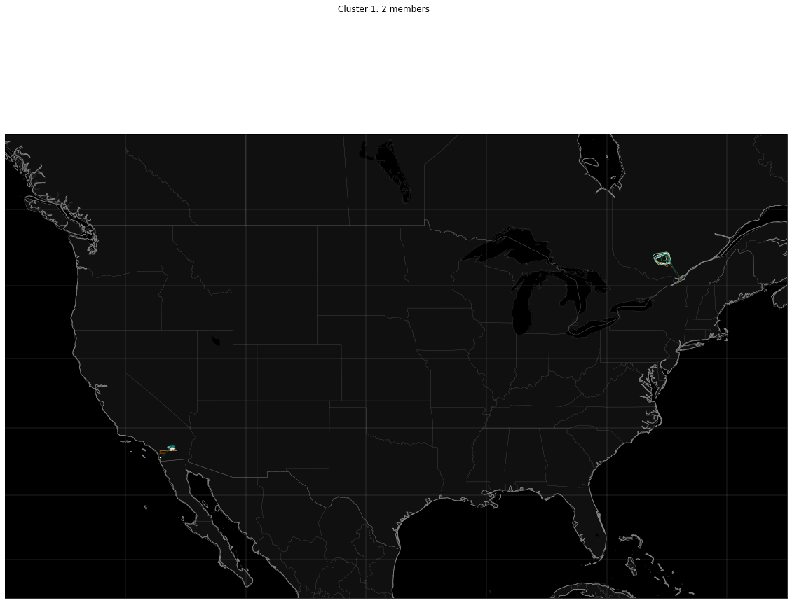
RESULT: Cluster sizes:
Outliers: 28
Cluster 1: 2

Cluster Visualization

You can use pyplot to see your clusters that were created

from tracktable.render import paths
from tracktable.domain import terrestrial
from tracktable.render import mapmaker
from matplotlib import pyplot

sorted_ids = sorted(clusters.keys())
for cluster_id in sorted_ids:
    # Set up the canvas and map projection
    figure = pyplot.figure(figsize=[20, 15])
    axes = figure.add_subplot(1, 1, 1)
    (mymap, map_actors) = mapmaker.mapmaker(domain = 'terrestrial', map_name='region:conus')
    paths.draw_traffic(traffic_map = mymap, trajectory_iterable = clusters[cluster_id], transform=cartopy.crs.PlateCarree())
    figure.suptitle('{}: {} members'.format(cluster_name(cluster_id),
                                           len(clusters[cluster_id])))
    pyplot.show()

/home/docs/checkouts/readthedocs.org/user_builds/tracktable/conda/v1.4.1.1/lib/python3.7/site-packages/cartopy/io/__init__.py:260: DownloadWarning: Downloading: https://naciscdn.org/naturalearth/110m/physical/ne_110m_land.zip
  warnings.warn('Downloading: {}'.format(url), DownloadWarning)
/home/docs/checkouts/readthedocs.org/user_builds/tracktable/conda/v1.4.1.1/lib/python3.7/site-packages/cartopy/io/__init__.py:260: DownloadWarning: Downloading: https://naciscdn.org/naturalearth/110m/physical/ne_110m_ocean.zip
  warnings.warn('Downloading: {}'.format(url), DownloadWarning)
/home/docs/checkouts/readthedocs.org/user_builds/tracktable/conda/v1.4.1.1/lib/python3.7/site-packages/cartopy/io/__init__.py:260: DownloadWarning: Downloading: https://naciscdn.org/naturalearth/110m/physical/ne_110m_lakes.zip
  warnings.warn('Downloading: {}'.format(url), DownloadWarning)
/home/docs/checkouts/readthedocs.org/user_builds/tracktable/conda/v1.4.1.1/lib/python3.7/site-packages/cartopy/io/__init__.py:260: DownloadWarning: Downloading: https://naciscdn.org/naturalearth/10m/cultural/ne_10m_admin_1_states_provinces_lakes.zip
  warnings.warn('Downloading: {}'.format(url), DownloadWarning)
/home/docs/checkouts/readthedocs.org/user_builds/tracktable/conda/v1.4.1.1/lib/python3.7/site-packages/cartopy/io/__init__.py:260: DownloadWarning: Downloading: https://naciscdn.org/naturalearth/10m/cultural/ne_10m_admin_0_boundary_lines_land.zip
  warnings.warn('Downloading: {}'.format(url), DownloadWarning)
/home/docs/checkouts/readthedocs.org/user_builds/tracktable/conda/v1.4.1.1/lib/python3.7/site-packages/cartopy/io/__init__.py:260: DownloadWarning: Downloading: https://naciscdn.org/naturalearth/50m/physical/ne_50m_coastline.zip
  warnings.warn('Downloading: {}'.format(url), DownloadWarning)