Tutorial 5-A: Interactive Trajectory Visualization
In [1]:
import tracktable.examples.tutorials.tutorial_helper as tutorial
from datetime import timedelta
Purpose
The next three notebooks demonstrate how to use Tracktable’s internal rendering functions to visualize trajectories. Tracktable has numerous rendering methods, and not all are shown here. A comprehensive rendering user guide can be found in the Tracktable documentation: https://tracktable.readthedocs.io/en/latest/user_guides/python/rendering.html
We break up this tutorial into three parts, each with its own notebook. Tutorial 5-A details interactive trajectory visualization. Tutorial 5-B details static trajectory visualization. Tutorial 5-C details visualization with heat maps (both static and interactive).
IMPORTANT: When rendering trajectories interactively, the memory required to render large lists of trajectories may cause your browser to shut down. Try rendering smaller datasets first and work up from there to test your browser’s capacity.
Let’s start with a list of trajectories.
We will use the provided example data \(^1\) for this tutorial. For brevity, the function below reads our trajectories from a .traj file into a Python list, as was demoed in Tutorial 4.
In [2]:
trajectories = tutorial.get_trajectory_list()
Loading Trajectories: 279 trajectory [00:00, 4887.77 trajectory/s]
[2025-06-08 20:58:37.903356] [0x00000001f1aadf00] [info] Read a total of 279 trajectories.
In [3]:
from tracktable.render.render_trajectories import render_trajectories, render_trajectories_separate
Default Rendering
Let’s start by rendering just the first trajectory in our list.
In [4]:
trajectory = trajectories[0]
By default, trajectories are rendered in Folium, allowing you to scroll and zoom. Each trajectory is hashed to a color using its object_id string. Each trajectory’s color starts out dark at its oldest end and grows progressively lighter through time. The end of each trajectory (its most recent point) is marked with a white dot.
In [5]:
render_trajectories(trajectory)
Out[5]:
Now let’s render a list of fifteen trajectories together.
In [6]:
fifteen_trajectories = trajectories[5:20]
In [7]:
render_trajectories(fifteen_trajectories)
Out[7]:
We can also render a list of trajectories separately. This will display one Folium window for each trajectory.
In [8]:
three_trajectories = trajectories[10:13]
In [9]:
render_trajectories_separate(three_trajectories)
If there are a specific object’s trajectories that we wish to render, we can select them by the object ID.
In [10]:
render_trajectories(trajectories, obj_ids='367782880')
Out[10]:
… or select several object IDs.
In [11]:
render_trajectories(trajectories, obj_ids=['367782880', '367740750'])
Out[11]:
Animation
Set animate to ‘True’ to animate the trajectories.
With animations you can:
Adjust the speed of animation by dragging the FPS (frames per second) slider.
Pause (⏸️) the animation and use the time slider to manually advance the animation.
Click the forward (⏩) or backward (⏪) arrows (to the right and left of the play/pause (⏸️) icon) to advance by a single frame in either direction.
Toggle whether or not the animation repeats when finished by clicking the loop button to the right of the forward arrow (⏩).
Click Play (▶️) to resume the animation after pausing it.
In [12]:
render_trajectories(trajectories[27], animate=True)
Out[12]:
To get faster animation, decrease the anim_display_update_interval value in the call to render_trajectories. This is the real-world time between updates. In this case we are rendering an update on the map every 50 milliseconds. The example above showed an update every 200 milliseconds (five times per second). You can also show the individual trajectory points in the animation by providing show_points=True as an argument.
In [ ]:
render_trajectories(trajectories[27],
animate=True,
anim_display_update_interval=timedelta(microseconds=50000),
show_points=True)
You can control how quickly time advances in the animation with the timestamp update step argument. The display update interval (anim_display_update_interval) is how often the display will update; the timestamp update step (anim_timestamp_update_step) is how far the clock advances with each update.
For example, suppose that you have 100 hours of data sampled once per hour. The default value for the timestamp update step (one minute) would produce a very slow animation. By specifying anim_timestamp_update_step = timedelta(minutes=4) you can speed it up by a factor of four.
This next animation will complete in the same time as the previous one. In the previous example, we advanced time one minute at each update and rendered one update every 50 milliseconds (50,000 microseconds). The next example renders new updates every 200 milliseconds (four times more slowly) but moves time forward four minutes per update (four times more quickly).
In [13]:
render_trajectories(trajectories[27],
animate=True,
anim_timestamp_update_step=timedelta(minutes=4))
Out[13]:
By default, trajectory animations show the entirety of each trajectory’s history from its start up to the current update’s timestamp. You can decrease this using the anim_trail_duration argument.
The following example will show only the previous 5 minutes of data for our example trajectory at each step in the animation.
In [14]:
render_trajectories(trajectories[27],
animate=True,
anim_trail_duration=timedelta(minutes=5))
Out[14]:
Changing the Back End
By default, Tracktable renders trajectories using Folium when in Jupyter notebooks in order to produce interactive maps. We can change this to Cartopy to produce static images if we prefer. This is demonstrated in Tutorial 5-B. Static images are a good choice when you have too much data to render interactively.
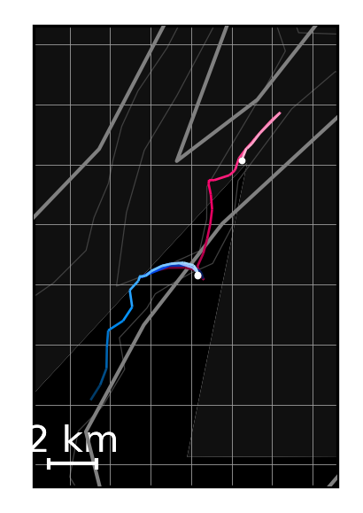
Here we draw the same three trajectories we used earlier but with the Cartopy back end instead of Folium. In this particular example the coastlines are much lower-resolution than in the tiles Folium uses. You can see how to change this in Tutorial 5-B.
In [15]:
render_trajectories(three_trajectories,
backend='cartopy',
scale_length_in_km=2)
Out[15]:
<GeoAxes: >
Changing the Map
In Folium, the map background is downloaded on the fly from a tile server. We use the tiles keyword argument to render_trajectories to select between several tile servers built into Folium.
Here are the available options:
CartoDBDark_Matter(the default)OpenStreetMapsStamenTerrainStamenTonerStamenWatercolorCartoDBPositron
In [16]:
render_trajectories(fifteen_trajectories,
tiles='CartoDBPositron')
Out[16]:
You can also specify a map tile server by URL. You will need to specify the keyword argument attr, the attribution string.
In [17]:
render_trajectories(fifteen_trajectories,
tiles='http://server.arcgisonline.com/ArcGIS/rest/services/NatGeo_World_Map/MapServer/tile/{z}/{y}/{x}', attr='ESRI')
Out[17]:
By default, the map will initially be zoomed to fit all trajectories, but a specific bounding box can be specified. Note that the format of the bounding box should be [min_longitude, min_latitude, max_longitude, max_latitude].
In [18]:
render_trajectories(fifteen_trajectories,
map_bbox=[-75.1, 39.9, -73.2, 40.9])
Out[18]:
Changing Trajectory Rendering Styles
By default the line width is 2.4, but can be adjusted to any positive number.
In [19]:
render_trajectories(trajectory, linewidth=10)
Out[19]:
We can render multiple trajectories in one solid color. We specify that color by passing a string to the line_color parameter. We choose plum here, but any HTML-style color will work.
In [20]:
render_trajectories(three_trajectories,
line_color='plum')
Out[20]:
Alternatively, we can pass in the color as a hex string of the format #RRGGBBAA where RR (red), GG (green) and BB (blue) are values from 0 to 255 as two hex digits each. The last two hex digits AA (alpha) are optional and control opacity (e.g. FF = 100% and 00 = 0%).
In [21]:
render_trajectories(three_trajectories,
line_color='#E6E6E650')
Out[21]:
The trajectories can also be colored using a Matplotlib colormap.
A complete list of colormaps can be viewed here: https://matplotlib.org/stable/tutorials/colors/colormaps.html.
In [22]:
render_trajectories(three_trajectories,
color_map='plasma')
Out[22]:
You can even define your own color maps.
In [23]:
import matplotlib
import numpy as np
In [25]:
# start with the matplotlib 'Blues colormap'
blues_map = matplotlib.colormaps.get_cmap('Blues')
# convert a matplotlib colormap to a numpy matrix of size (100, 4) composed of 100 colors each represented
# by their RGB representation (4 numbers - red, green, blue, and opacity scaled between 0 and 1)
newcolors = blues_map(np.linspace(0, 1, 100))
# define pink using RGB representation
pink = np.array([248/256, 24/256, 148/256, 1]) # R G B Opacity
# use pink for takeoff by setting the first ~10% of trajectory to use the color pink
newcolors[:10, :] = pink
render_trajectories(three_trajectories, color_map = matplotlib.colors.ListedColormap(newcolors))
Out[25]:
Controlling Trajectory Color
To select the feature that will be used for trajectory color, create a trajectory scalar generator: a function that takes a single argument (a TrajectoryPoint) and returns some quantity of interest such as heading, speed, altitude, climb rate, or any other number you might want to display as a color.
Pass the scalar generator to render_trajectories() with the trajectory_scalar_generator=my_scalar_function keyword argument. You will probably also want to set minimum and maximum values for the scalar using the color_scale argument as demonstrated below.
In [26]:
# This example uses the heading (bearing) from one point to the next
# as the trajectory color. You could also use vmin=0, vmax=359 if
# your trajectories use the entire possible range of headings.
#
# The Tracktable function bearing() returns headings in the range
# [0, 359] rather than [-180, 180].
from tracktable.core.geomath import bearing
def heading_generator(trajectory):
# calculate bearing of each linear segment of the trajectory
return [bearing(trajectory[i], trajectory[i+1]) for i in range(len(trajectory)-1)]
render_trajectories(three_trajectories,
trajectory_scalar_generator=heading_generator,
color_scale=matplotlib.colors.Normalize(vmin=36, vmax=349))
Out[26]:
Controlling Trajectory Line Width
You can control trajectory line width in the same way. Create a function that takes a TrajectoryPoint as its single argument and returns a number to be used as the trajectory’s width. Pass that function to render_trajectories() with the trajectory_linewidth_generator=my_width_function keyword argument.
In the example below we will use a built-in method that will widen the line as the trajectory progresses so that it is narrowest at its oldest point and widest at its newest point.
In [27]:
from tracktable.render.map_processing.common_processing import progress_linewidth_generator
render_trajectories(trajectory, trajectory_linewidth_generator=progress_linewidth_generator)
Out[27]:
Overriding Random Color Selection
You can render many trajectories in a single color by providing the gradient_hue keyword argument. Its value can be a color name, an RGB hex string, or a float from 0 to 1.
In [28]:
render_trajectories(three_trajectories, gradient_hue=0.2)
Out[28]:
Different trajectories in different colors
The line_color, color_map, and gradient_hue arguments all take lists as well as single values. The renderer will repeat the list if there are more trajectories than list elements.
In [29]:
render_trajectories(three_trajectories, line_color=['red', 'blue', 'green'])
Out[29]:
In [30]:
render_trajectories(three_trajectories, color_map=['plasma', 'viridis', 'gray'])
Out[30]:
In [31]:
render_trajectories(three_trajectories, gradient_hue=[0.1, 0.5, 0.9])
Out[31]:
Rendering Trajectory Points
So far, we have only rendered the lines for the trajectories plus a white dot at the newest end of the trajectory. We can also render the locations of the trajectory points along the way by passing show_points=True to render_trajectories().
In [32]:
render_trajectories(trajectory, show_points=True)
Out[32]:
The color and size of the dots at the trajectory points can be changed with the point_color and point_size keyword arguments.
In [33]:
render_trajectories(trajectory, show_points=True, point_color='red', point_size=3)
Out[33]:
The dot_size and dot_color keyword arguments affect only the head of the trajectory (the most recent point rendered).
In [34]:
render_trajectories(trajectory, show_points=True, dot_color='red', dot_size=3)
Out[34]:
We can turn off the dot at the end of the trajectory with the show_dot parameter.
In [35]:
render_trajectories(trajectory, show_dot=False)
Out[35]:
To see a trajectory point’s properties in a popup when a trajectory point is clicked, send a list of the desired properties to point_popup_properties.
In [36]:
render_trajectories(trajectory, show_points=True, point_popup_properties = ['eta', 'heading'])
Out[36]:
Exporting Renderings
If you come across a rendering you really like, you can save the trajectories as an html file (default filename is trajs-timestamprange.html).
In [ ]:
render_trajectories(fifteen_trajectories, save=True, filename='my_favorite_trajectories.html')
\(^1\) Bureau of Ocean Energy Management (BOEM) and National Oceanic and Atmospheric Administration (NOAA). MarineCadastre.gov. AIS Data for 2020. Retrieved February 2021 from marinecadastre.gov/data. Trimmed down to the first hour of June 30, 2020, restricted to in NY Harbor.