Rendering
Now we come to the fun part of Tracktable: making images and movies from data.
Tracktable supports three kinds of visualization:
A heatmap (2D histogram)
A trajectory map (lines/curves drawn on the map)
A trajectory movie
Note
Visualization in tracktable can be static or interactive
depending on the backend selected for render_trajectories,
cartopy or folium respectively.
Note
We render heatmaps directly from points. Trajectory maps and movies require assembled trajectories.
In all cases we render points into a 2D projection. In this section of the user’s guide we will discuss rendering onto a map projection. The procedure for rendering points in Cartesian space is very similar and will be documented Real Soon Now.
We use the Cartopy toolkit for the map projection and Matplotlib for the actual rendering.
Note
In order to view the images being rendered, either output the image to a file, execute the code in a notebook, or otherwise ensure your environment can launch an image viewing application.
Setting Up a Map
The easiest way to create and decorate a map is with the
tracktable.render.render_map.render_map() function. It can
create maps of common (named) areas of the world, regions surrounding
airports, ports, and user-specified regions.
Predefined Region Map
Here’s an example that will create a map of Australia with coastlines and longitude/latitude graticules rendered every 2 degrees.
 1from tracktable.render.render_map import render_map
 2from matplotlib import pyplot
 3
 4f = pyplot.figure(figsize=(8, 6), dpi=100)
 5
 6(mymap, initial_artists) = render_map(domain='terrestrial',
 7                                     map_name='region:australia',
 8                                     draw_coastlines=True,
 9                                     draw_countries=False,
10                                     draw_states=False,
11                                     draw_lonlat=True,
12                                     lonlat_spacing=2,
13                                     lonlat_linewidth=0.5)
We always return two values from render_map. The first is the
cartopy.mpl.geoaxes instance that will convert
points between world coordinates (longitude/latitude) and map
coordinates. The second is a list of Matplotlib artists
that define all the decorations added to the map.
There are several predefined map areas. Their names can be retrieved
by programmatically calling tracktable.render.maps.available_maps()
and for the convience of the user guide these maps are:
region:conusregion:europeregion:worldregion:north_americaregion:south_americaregion:australia
Hint
If you would like to have a region included please send us its name and longitude/latitude bounding box. We will gladly add it to the next Tracktable release. Contact us using the contact information listed under the Tracktable Contacts
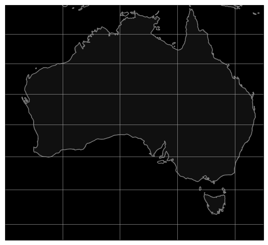
This map of Australia was generated by passing the map name
australia to render_map.
Predefined Airport Map
This next example will render a 200x200 km area around Boston’s Logan International Airport (BOS). Coastlines will be drawn with an extra-thick (2-point-wide) blue line. US state borders will be drawn in red. Land will be filled in grey. Water will be filled in black. BOS will be marked with a large red dot. We use high-resolution borders since we’re zoomed in fairly far.
 1from tracktable.render.render_map import render_map
 2from matplotlib import pyplot
 3
 4f = pyplot.figure(figsize=(8, 6), dpi=100)
 5(mymap, initial_artists) = render_map(domain='terrestrial',
 6                                     map_name='airport:BOS',
 7                                     draw_coastlines=True,
 8                                     draw_countries=False,
 9                                     draw_states=True,
10                                     draw_lonlat=True,
11                                     lonlat_spacing=2,
12                                     lonlat_linewidth=0.5,
13                                     land_fill_color='#505050',
14                                     land_resolution='50m',
15                                     coastline_color='blue',
16                                     coastline_linewidth=2,
17                                     coastline_resolution='10m',
18                                     ocean_resolution='50m',
19                                     state_color='red',
20                                     state_linewidth=1,
21                                     region_size=(200, 200),
22                                     draw_airports=True,
23                                     airport_dot_size=20,
24                                     airport_color='red')
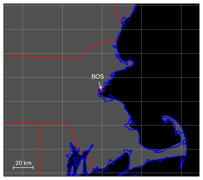
This map of the area around Boston’s Logan International Airport was generated by
passing the map name airport:BOS to render_map. The dot representing the airport
is generated by setting the draw_airports to True.
Note
The resolution of the borders in the generated image can be increased or
decreased by setting the country_resolution, state_resolution, coastline_resolution,
land_resolution, ocean_resolution and lake_resolution parameters.
Predefined Port Map
This next example will render a 200x200 km area around the port of Seattle. Coastlines will be drawn with an extra-thick (2-point-wide) blue line. US state borders will be drawn in red. Land will be filled in grey. Water will be filled in black. The Port of Seattle will be marked with a large red dot. We use high-resolution borders since we’re zoomed in fairly far.
 1from tracktable.render.render_map import render_map
 2from matplotlib import pyplot
 3
 4f = pyplot.figure(figsize=(8, 6), dpi=100)
 5(mymap, initial_artists) = render_map(domain='terrestrial',
 6                                     map_name='port:seattle',
 7                                     draw_coastlines=True,
 8                                     draw_countries=False,
 9                                     draw_states=True,
10                                     draw_lonlat=True,
11                                     lonlat_spacing=2,
12                                     lonlat_linewidth=0.5,
13                                     land_fill_color='#505050',
14                                     land_resolution='50m',
15                                     coastline_color='blue',
16                                     coastline_linewidth=2,
17                                     coastline_resolution='10m',
18                                     ocean_resolution='50m',
19                                     state_color='red',
20                                     state_linewidth=1,
21                                     region_size=(200, 200),
22                                     draw_ports=True,
23                                     port_dot_size=20,
24                                     port_color='red')
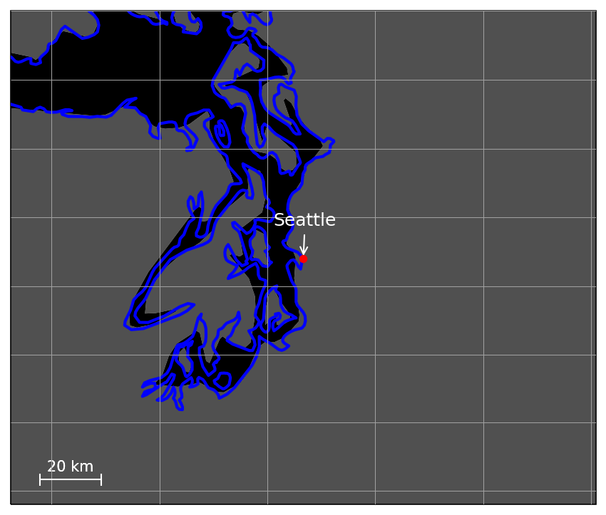
This map of the area around the Port of Seattle was generated by
passing the map name port:seattle to render_map. The dot representing the port
is generated by setting the draw_ports to True.
Note
The resolution of the borders in the generated image can be increased or
decreased by setting the country_resolution, state_resolution, coastline_resolution,
land_resolution, ocean_resolution and lake_resolution parameters.
Predefined City Map
Note
This functionality will be implemented in a future release.
Custom Map
If we want a map that does not correspond to any of the predefined
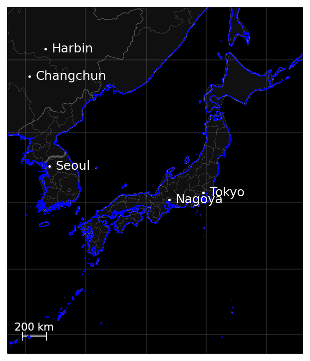
ones then we can use the custom map type. This example will create
a map of Japan and the Korean Peninsula with all cities labeled whose
population is larger than 2 million.
 1from tracktable.render.render_map import render_map
 2from matplotlib import pyplot
 3
 4f = pyplot.figure(figsize=(8, 6), dpi=100)
 5
 6# Bounding box is [longitude_min, latitude_min, longitude_max, latitude_max]
 7(mymap, initial_artists) = render_map(domain='terrestrial',
 8                                     map_name='custom',
 9                                     map_bbox = [123.5, 23.5, 148, 48],
10                                     draw_cities_larger_than=2000000)
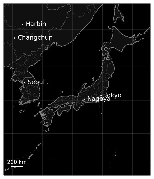
This map was generated by passing the map name custom and a
longitude/latitude bounding box to render_map.
Note
To define a map area that crosses the discontinuity at longitude +/- 180 degrees, use coordinates that wrap around beyond 180. The bounding boxes (-200, 0, -160, 40) and (160, 0, 200, 40) both define a region that extends from 0 to 40 degrees latitude and 20 degrees to either side of 180 degrees longitude.
Shorelines, Rivers, Borders
Shoreline, river and border gemotry objects can be added to a custom or predefined map. This is as simple as passing in the appropriate render flag along with zero or more specific polygons or bounding boxes to render. This example will use the same map creation logic from the section above but with the addition of shorelines. Rivers and borders follow the same conventions shown in this example.
 1from tracktable.render.render_map import render_map
 2from matplotlib import pyplot
 3
 4f = pyplot.figure(figsize=(8, 6), dpi=100)
 5
 6# Bounding box is [longitude_min, latitude_min, longitude_max, latitude_max]
 7(mymap, artists) = render_map.render_map(domain='terrestrial',
 8                                     map_name='custom',
 9                                     map_bbox = [123.5, 23.5, 148, 48],
10                                     draw_cities_larger_than=2000000,
11                                     scale_length_in_km=200,
12                                     draw_shorelines=True,
13                                     shoreline_color='blue',
14                                     shoreline_fill_polygon=False)
This map was generated by passing the map name custom and a
longitude/latitude bounding box to render_map as well as setting
the draw_shorelines flag to True.
Cartesian
Similar to the terrestrial maps described above Tracktable contains the ability to render map projections in the Cartesian domain. The example below will generate a blank cartesian2d that can be filled with points or trajectories.
1from tracktable.render.render_map import render_map
2from matplotlib import pyplot
3
4f = pyplot.figure(figsize=(8, 6), dpi=100)
5
6(mymap, initial_artists) = render_map(domain='cartesian2d',
7                                     map_name='custom',
8                                     map_bbox = [-100, -100, 100, 100])

This map was generated by passing the domain cartesian2d,
map name custom and a longitude/latitude bounding box to render_map.
Rendering Onto the Map
Since Tracktable uses Matplotlib as its
underlying renderer you can immediately render almost anything you
want on top of a map. Remember, however, that Matplotlib does not
know about the map projection. In order to draw things that will be
properly registered onto the map you need to use the
cartopy.mpl.geoaxes instance that we
got earlier when we set up our map using render_map. By calling the map
instance as if it were a function you can convert coordinates from
world space (longitude/latitude) to axis space (arbitrary coordinates
established by Matplotlib).
There are many ways to draw things like contours, points, curves, glyphs and text directly onto the map. Please refer to the cartopy example gallery for demonstrations. Tracktable provides code to render two of the most common use cases for trajectory data: heatmaps (2D histograms) and trajectory maps.
Heat Maps
A heat map (Wikipedia page) is a two-dimensional histogram – that is, a density plot. We use heat maps to illustrate the density of points that compose a set of trajectories. We are typically looking for areas of high traffic and areas of coverage.
This release of Tracktable supports heat maps rendered on top of
geographic maps using the
tracktable.render.histogram2d.geographic class. You
must call it with at least two arguments – a
cartopy.mpl.geoaxes
instance and an iterable of points. Other optional arguments
will let you control the histogram bin size,
color map and where on the map the heatmap is rendered.
A start-to-finish example of how to load points and render a heat map can be found on the heatmap example page.
Note
The tracktable.render.histogram2d.geographic
heat map generator only traverses its input data once to keep memory
requirements low. You can safely use it with point sets too
large to load into memory at once.
Trajectory Maps
A trajectory map is an ordinary map with one or more trajectories drawn on it. We may want to decorate a trajectory with any of the following:
Colors defined as a function of some quantity computed for the trajectory such as speed, turn rate or altitude
Variable line widths (such as a trajectory that is broad at its head and narrow at its tail)
A dot of some color and size at the head of the trajectory to mark the object’s actual position
A label at the head of the trajectory to display an object ID
All of this is packaged into the function draw_traffic
in the tracktable.render.paths module.
Note
The argument names for that function are slightly
misleading. Pay careful attention to the documentation for
that function. Specifically, the arguments
trajectory_linewidth_generator and
trajectory_scalar_generator seem to indicate by their
names that you must compute the linewidths and scalars at
render time. This is fine for single images. For movies,
we find it more useful to compute as much as we can before
rendering and then pass an accessor function in as the
generator.
Similar to heat maps, a start-to-finish example on how to load points and generate trajectory maps can be found on the trajectory map example page.
Making Movies
To a first approximation, making a movie is the same as making a single image many, many times. The part that takes some care is minimizing the number of times we perform expensive operations such as loading data and configuring/decorating a map.
As with heat maps and trajectory maps a start-to-finish example how to load points and generate trajectory movies can be found on the movie rendering example page.