Tutorial 5-D: Trajectory Visualization For Print
In [24]:
# TODO: Clean up this Tutorial to make the others
Purpose: Generate trajectory images that are specifically designed for a paper/report
In [25]:
#This notebook demonstrates plotting trajectory figures for use in printed media / papers.

from tracktable.domain.terrestrial import TrajectoryPointReader
from tracktable.applications.assemble_trajectories import AssembleTrajectoryFromPoints
from tracktable.render.render_trajectories import render_trajectories_for_print
from tracktable.render.render_trajectories import render_trajectories_for_print_using_tiles
#from tracktable.algorithms.dbscan import compute_cluster_labels
from tracktable_data.data import retrieve
from datetime import timedelta
import cartopy
import cartopy.crs

data_filename = retrieve(filename='SampleFlightsUS.csv')
inFile = open(data_filename, 'r')
reader = TrajectoryPointReader()
reader.input = inFile
reader.comment_character = '#'
reader.field_delimiter = ','
reader.object_id_column = 0
reader.timestamp_column = 1
reader.coordinates[0] = 2
reader.coordinates[1] = 3

builder = AssembleTrajectoryFromPoints()
builder.input = reader
builder.minimum_length = 5
builder.separation_time = timedelta(minutes=10)

all_trajectories = list(builder)
INFO:tracktable.applications.assemble_trajectoriesAssembleTrajectoryFromPoints:New trajectories will be declared after a separation of None distance units between two points or a time lapse of at least 0:10:00 (hours, minutes, seconds).
INFO:tracktable.applications.assemble_trajectoriesAssembleTrajectoryFromPoints:Trajectories with fewer than 5 points will be discarded.
INFO:tracktable.applications.assemble_trajectoriesAssembleTrajectoryFromPoints:Done assembling trajectories. 30 trajectories produced and 1 discarded for having fewer than 5 points.
In [26]:
# Default behavior:
# Give it a list of trajectories and a filename.  Extension can be png, pdf, etc and it will output in correct format.
render_trajectories_for_print(all_trajectories[0], "myfig0.pdf")
In [27]:
#can change colormap to any supported by matplotlib.  We recommend default (viridis) or this one (cividis)
render_trajectories_for_print(all_trajectories[0], "myfig0.png", color_map='cividis')
In [28]:
#Depending on your track(s) you may need to adjust linewidth until it's wide enough to see well, but not too thick.
render_trajectories_for_print(all_trajectories[0], "myfig1.pdf", linewidth=1.5, draw_scale=False)

In [29]:
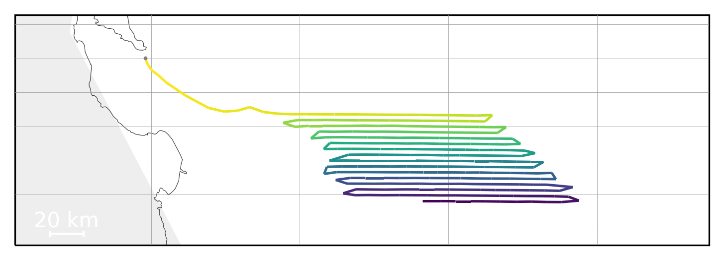
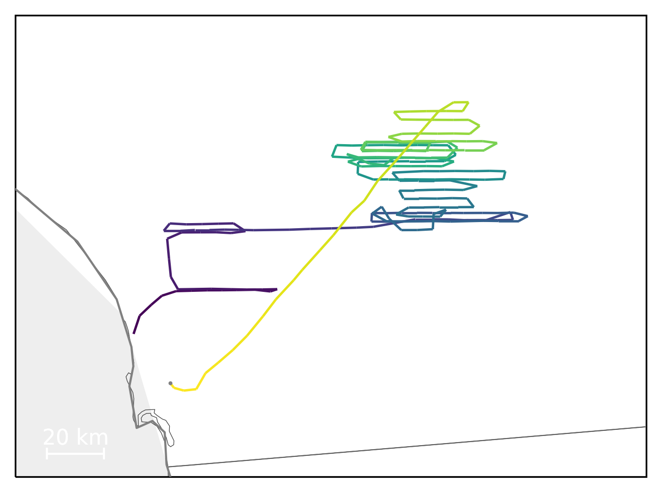
# There are multiple boarders (state and coastlines) that converge at the seashore.  You may want to turn off coastlines
render_trajectories_for_print(all_trajectories[4], "myfig4.pdf", draw_coastlines=False)
#other things you can tweak:
#                     draw_countries=True,
#                     draw_states=True,
#                     fill_land=True,
#                     fill_water=True,
#                     land_fill_color='#101010',
#                     water_fill_color='#000000',
#                     land_zorder=4,
#                     water_zorder=4,
#                     lonlat_spacing=10,
#                     lonlat_color='#A0A0A0',
#                     lonlat_linewidth=0.2,
#                     lonlat_zorder=6,
#                     coastline_color='#808080',
#                     coastline_linewidth=1,
#                     coastline_zorder=5,
#                     country_color='#606060',
#                     country_fill_color='#303030',
#                     country_linewidth=0.5,
#                     country_zorder=3,
#                     state_color='#404040',
#                     state_fill_color='none',
#                     state_linewidth=0.3,
#                     state_zorder=2,
#                     draw_largest_cities=None,
#                     draw_cities_larger_than=None,
#                     city_label_size=12,
#                     city_dot_size=2,
#                     city_dot_color='white',
#                     city_label_color='white',
#                     city_zorder=6,
#                     country_resolution='10m',
#                     state_resolution='10m',
#                     coastline_resolution='50m',
#                     land_resolution='110m',
#                     ocean_resolution='110m',
#                     lake_resolution='110m',
#                     map_bbox=None,
#                     map_projection=None,
#                     map_scale_length=None,
#                     region_size=None
In [30]:
#can turn off Lat/Lon lines
render_trajectories_for_print(all_trajectories[11], "myfig11.pdf", linewidth=1.4, draw_lonlat=False)
In [31]:
#You can set the size of the figure in inches (width,height) dpi defaults to 300
#unfortunately in this case the map will remain skinny, while the figure will be wide with lots of
#whitespace on both sides. (you may need to look at the output pdf to see the whitespace.)
render_trajectories_for_print(all_trajectories[13], "myfig13a.pdf", linewidth=.9, figsize=(3,2), draw_coastlines=False)

In [32]:
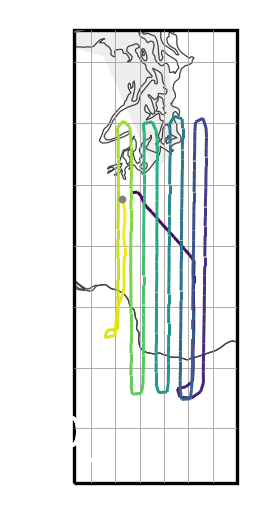
#To fix that extra whitespace (unless you manually crop) you can either adjust the figsize (see pdfs for comparison)
render_trajectories_for_print(all_trajectories[13], "myfig13b.pdf", linewidth=.9, figsize=(1,2), draw_coastlines=False)
In [33]:
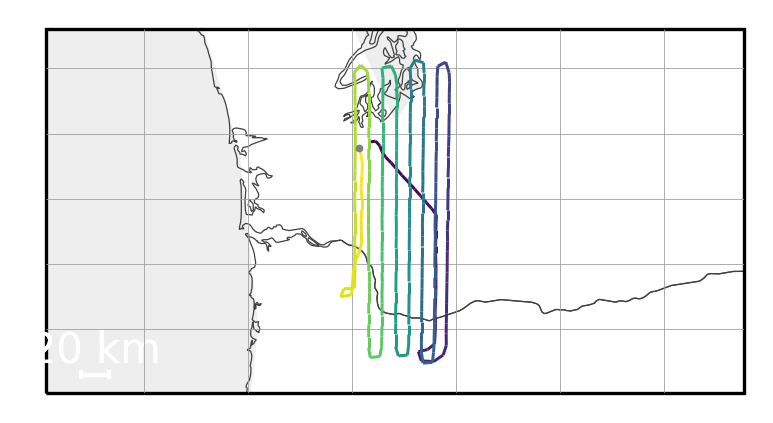
#Or, add extra "bounding box buffer" (width, height) to the map such that more map is shown.  (we hope to automate this at some point)
render_trajectories_for_print(all_trajectories[13], "myfig13c.pdf", linewidth=.9, figsize=(3,2), bbox_buffer=(2.7,.1), draw_coastlines=False)
In [34]:
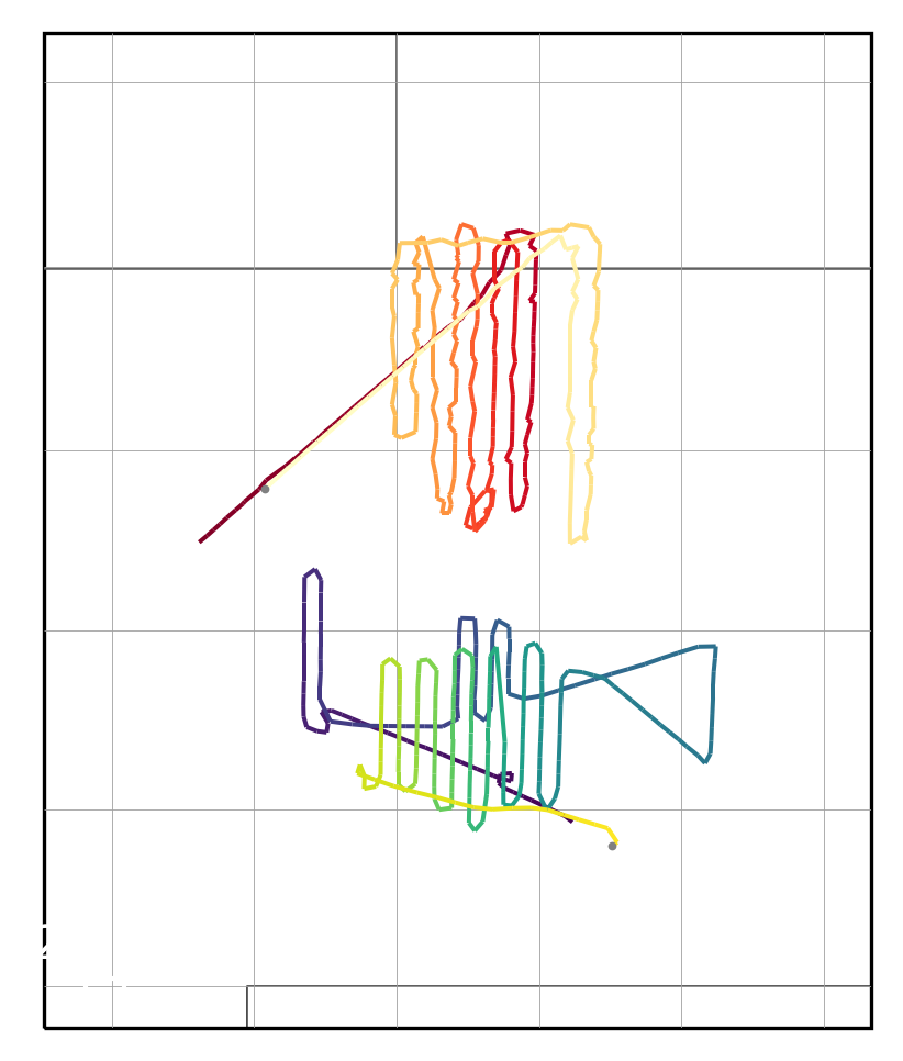
#If you wish to show multiple trajectories with different coloring here are some options:  Multiple color_maps (_r reverses the map)
render_trajectories_for_print(all_trajectories[14:16], "myfig14a.pdf", color_map=['viridis','YlOrRd_r'], linewidth=1.2)
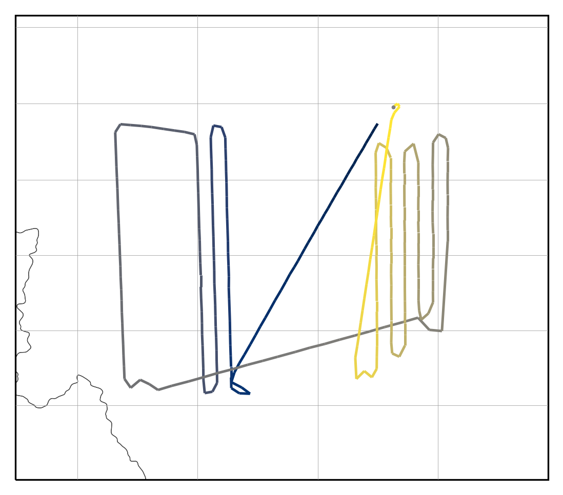
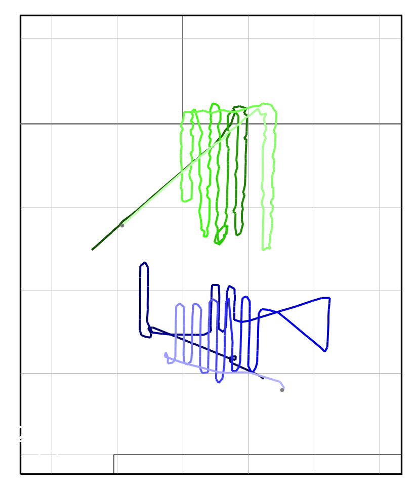
In [35]:
#you may specify the hue for a gradient (dark -> light) using a number (0-1) or a color name or a #RRGGBB color specification (see render_trajectories() for mor info)
render_trajectories_for_print(all_trajectories[14:16], "myfig14b.pdf", gradient_hue=['blue',.3], linewidth=1.2)
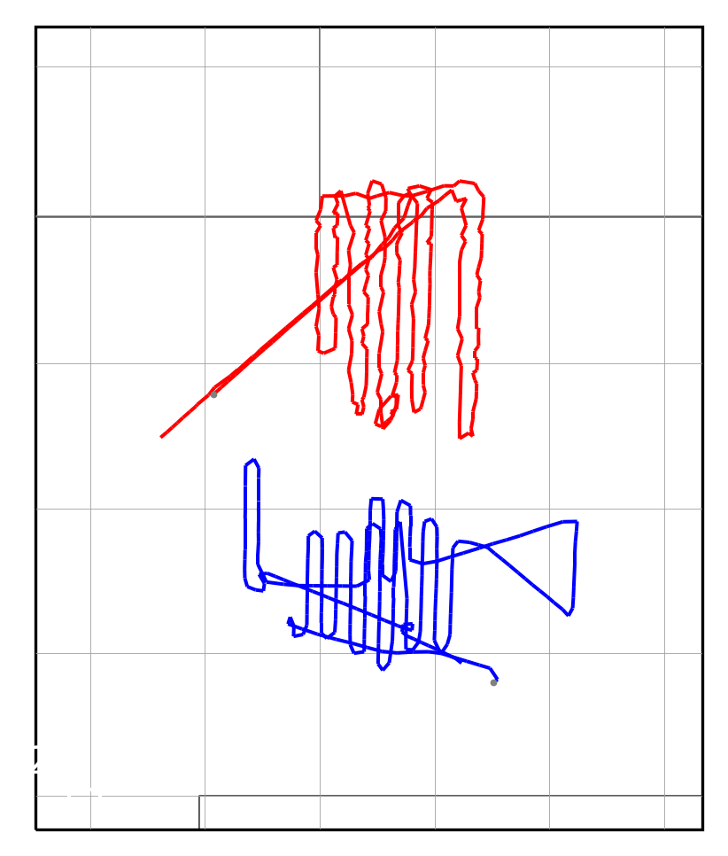
In [36]:
#you may specify a solid color for the lines
render_trajectories_for_print(all_trajectories[14:16], "myfig14c.pdf", line_color=['blue','red'], linewidth=1.2)
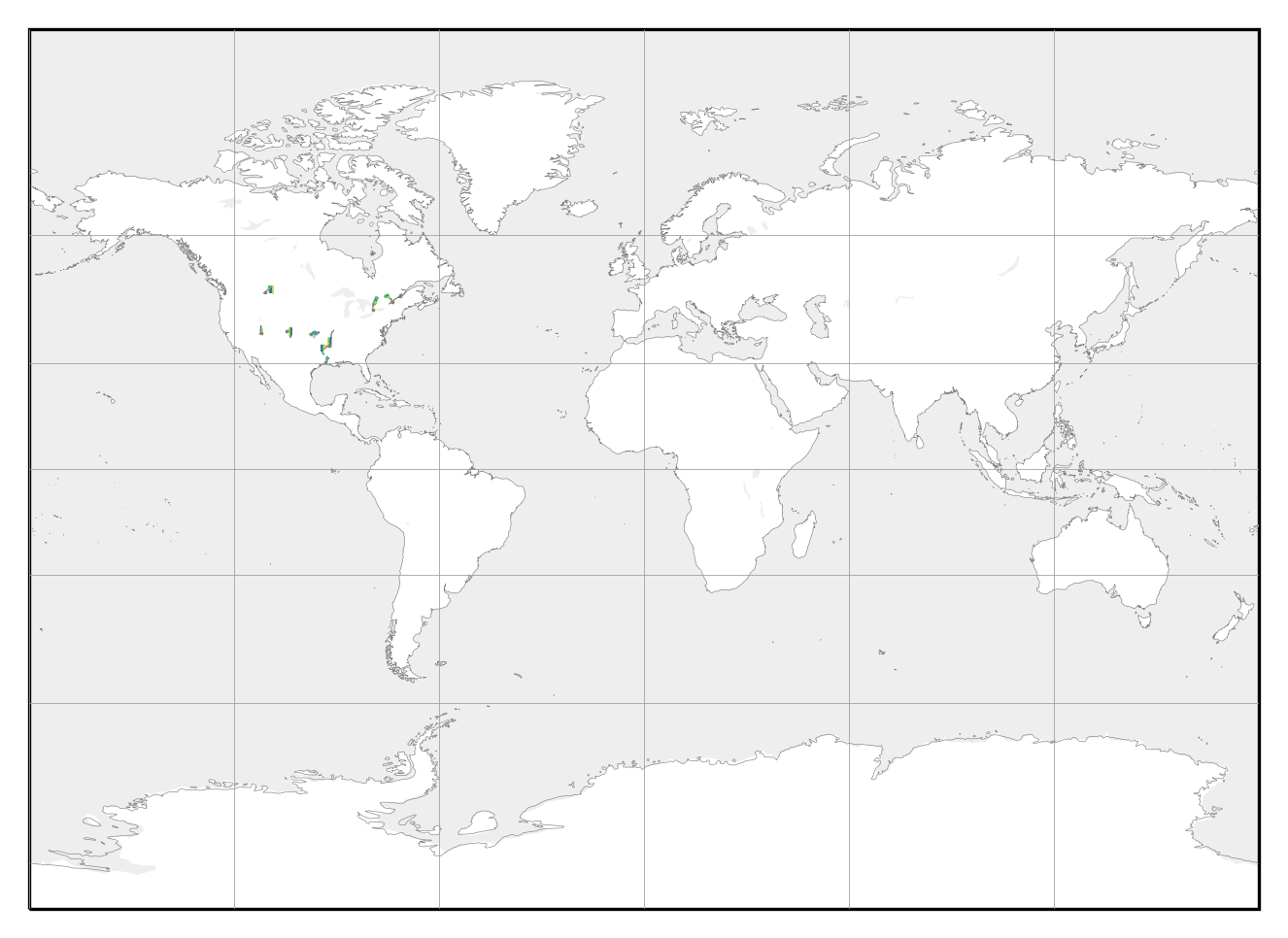
In [37]:
# You can specify a specific bounding box.  In this case entire world.
render_trajectories_for_print(all_trajectories[15:25], "myfig15a.pdf", map_bbox=[-179,-89,179,89], linewidth=.3, coastline_linewidth=.15, draw_countries=False, draw_states=False, dot_size=.05, draw_scale=False)
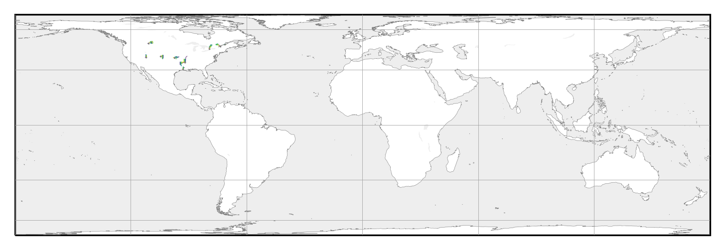
In [38]:
#You can specify a projection (LambertCylindrical)
# See options here: https://scitools.org.uk/cartopy/docs/latest/crs/projections.html
render_trajectories_for_print(all_trajectories[15:25], "myfig15b.pdf", map_projection=cartopy.crs.LambertCylindrical, map_bbox=[-179,-89,179,89], linewidth=.3, coastline_linewidth=.15, draw_countries=False, draw_states=False, dot_size=.05, draw_scale=False)
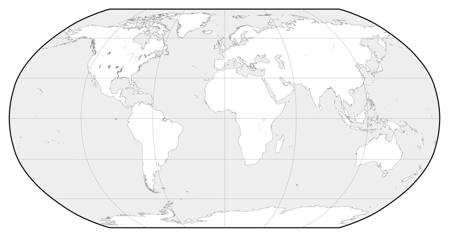
In [39]:
#if using a "global" projection and you want to see all of it, set map_global=True to use the limites of the projection
render_trajectories_for_print(all_trajectories[15:25], "myfig15c.pdf", map_global=True, map_projection=cartopy.crs.Robinson, linewidth=.3, coastline_linewidth=.15, draw_countries=False, draw_states=False, dot_size=.05)
In [40]:
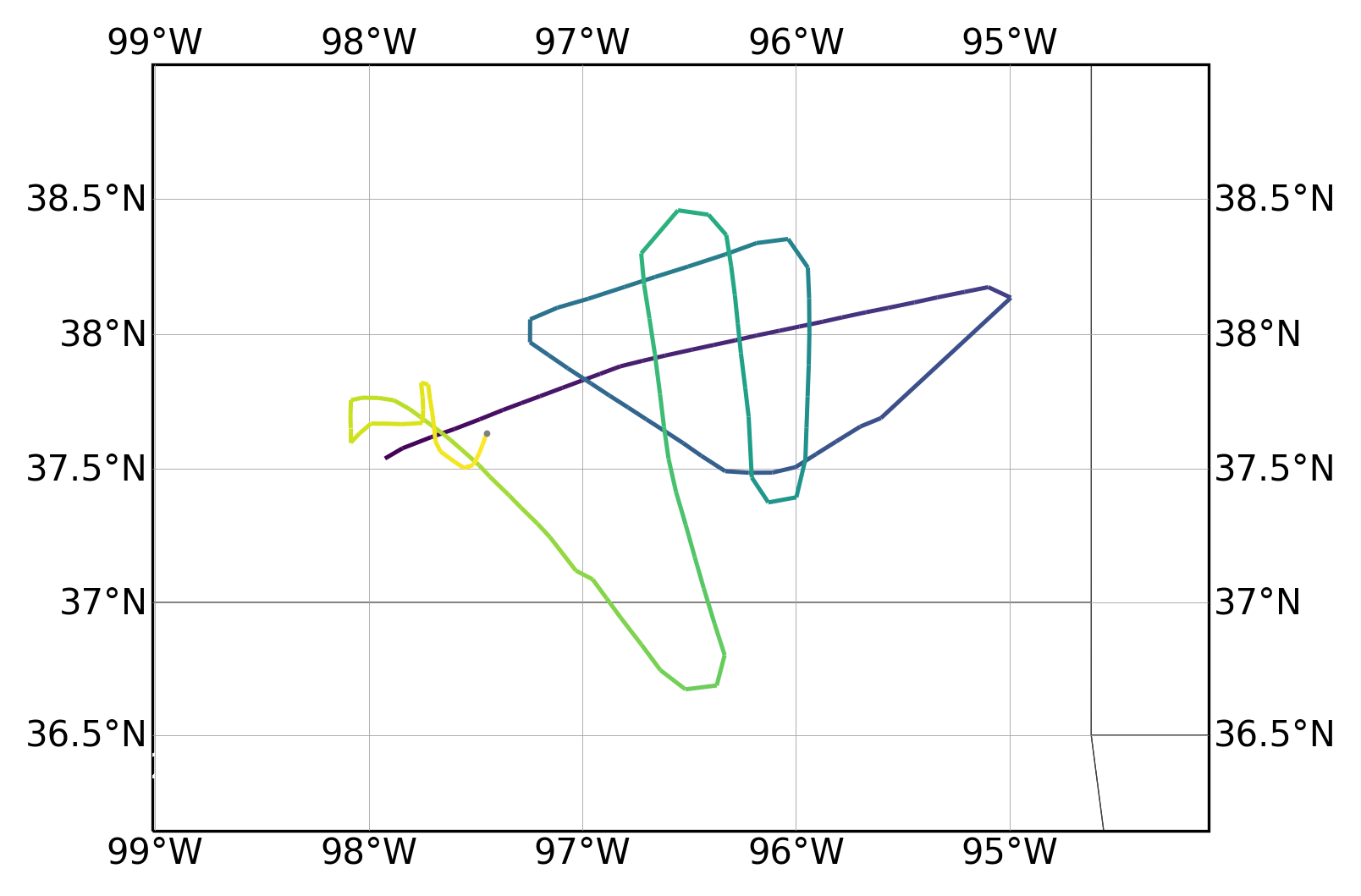
# You can add labels for lon/lat, only with certain projections.
# Only PlateCarree and Mercator plots currently support drawing labels for lon/lats.
#Recommended projection (Miller) does not support automatically drawing labels.
render_trajectories_for_print(all_trajectories[17], "myfig17.pdf", lonlat_labels=True, map_projection=cartopy.crs.Mercator)
In [41]:
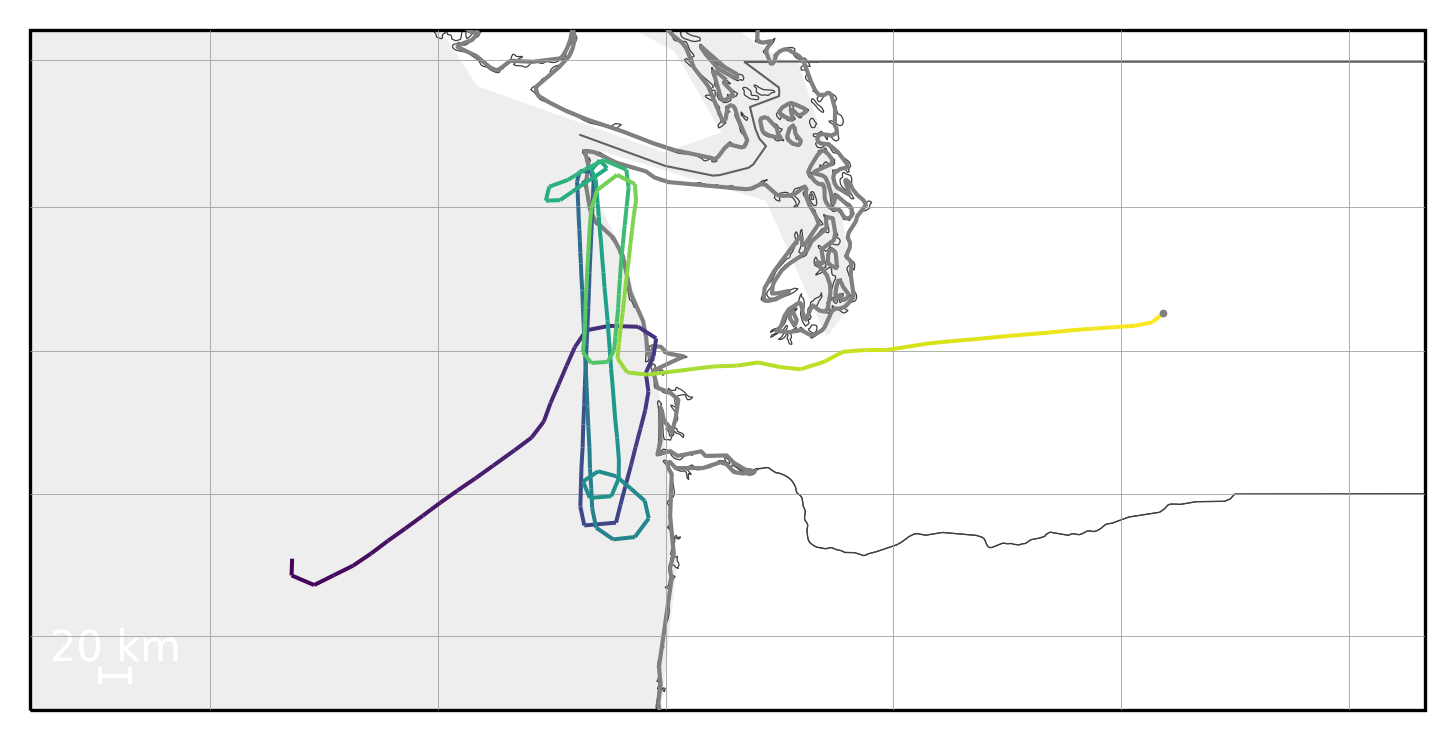
# The border resolution can be adjusted. (Low res)
#110m = low res, 50m = med res, 10m high res
render_trajectories_for_print(all_trajectories[25], "myfig25a.pdf", linewidth=1.2, border_resolution='110m')

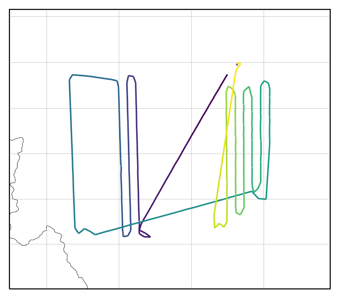
In [42]:
# The border resolution can be adjusted. (High res)
render_trajectories_for_print(all_trajectories[25], "myfig25b.pdf", linewidth=1.2, border_resolution='10m')
In [43]:
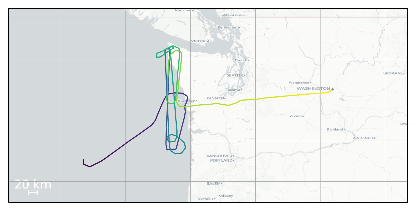
#using this method you can use map tiles instead of Cartopy geometry.
render_trajectories_for_print_using_tiles(all_trajectories[25], "myfig25c.pdf", linewidth=1.2)
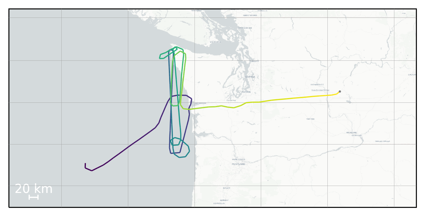
In [44]:
# You can change the zoom level
render_trajectories_for_print_using_tiles(all_trajectories[25], "myfig25d.pdf", linewidth=1.2, tiles_zoom_level=2)
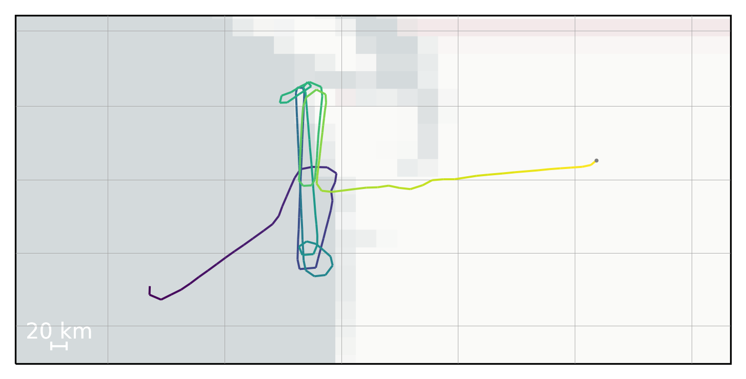
In [45]:
# And should adjust the zoom level until the label font is correclty sized.
render_trajectories_for_print_using_tiles(all_trajectories[25], "myfig25e.pdf", linewidth=1.2, tiles_zoom_level=7)