Tutorial 5-B: Static Trajectory Visualization

Purpose: Static images of trajectories are useful for publication and presentation since they do not require network access to fetch background tiles. They are also useful when rendering very large numbers of trajectories that might crash a web browser.

import tracktable.examples.tutorials.tutorial_helper as tutorial

Let’s start with a list of trajectories.

We will use the provided example data \(^1\) for this tutorial. For brevity, the function below reads our trajectories from a .traj file into a python list, as was demoed in Tutorial 4.

trajectories = tutorial.get_trajectory_list('tutorial-static-viz')

Loading Trajectories: 200 trajectory [00:00, 1292.93 trajectory/s]

[2025-06-09 01:06:23.350028] [0x00000001f1aadf00] [info]    Read a total of 200 trajectories.

Let’s work with 15 trajectories so that our visualizaitons render quickly.

fifteen_trajectories = trajectories[60:75]

from tracktable.render import render_map
from tracktable.render.map_processing import paths
import cartopy
import matplotlib
import matplotlib.pyplot as plt

Our static map choices are conus (continental United States), europe, north_america, south_america, australia, and world. These can be passed in as strings appended to region: in the map_name parameter of the mapmaker function.

A quick note about Jupyter notebooks. Jupyter will show you the state of the figure when you exit the cell in which you created it. You cannot apply different effects in different cells. To work around this, we put all our different effects in functions, then call those functions one after another in a single cell.

# Set up our canvas to be a 800x600 image (8x6 inches at 100 dpi).
figure = plt.figure(dpi=100, figsize=(8, 6))

# Set up our map projection to be the entire world.
(mymap, map_actors) = render_map.render_map(domain='terrestrial', map_name='region:world')

# Render the trajectories.
paths.draw_traffic(traffic_map=mymap, trajectory_iterable=fifteen_trajectories, transform=cartopy.crs.PlateCarree())

[<matplotlib.collections.LineCollection at 0x145cdf7a0>,
 <matplotlib.collections.PathCollection at 0x145b27380>]

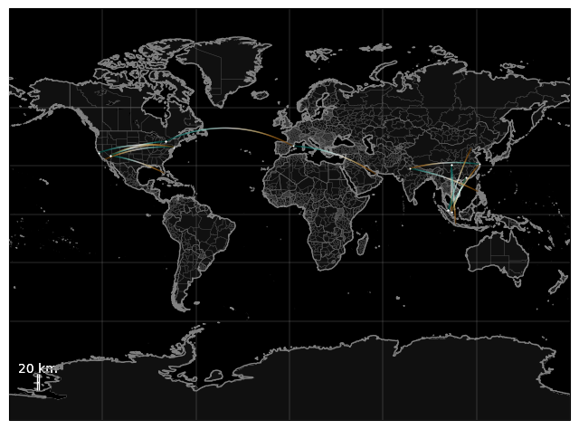
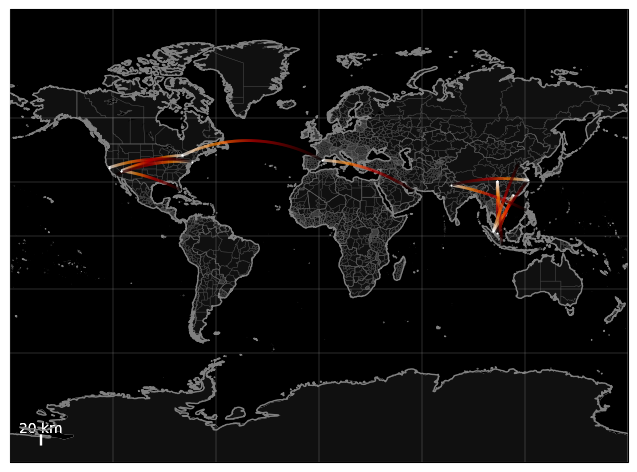
These trajectories are a bit hard to see. Let’s customize our rendering to make the trajectories easier to see:

1. Use color_map to get a red heat color.

2. Use linewidth to make the lines thicker.

3. Use dot_size to make the destination easier to see.

4. Use transform to define our cartopy projection.

# Set up our canvas to be a 800x600 image (8x6 inches at 100 dpi).
figure = plt.figure(dpi=100, figsize=(8, 6))

# Set up our map projection to be the entire world.
(mymap, map_actors) = render_map.render_map(domain='terrestrial',
                                        map_name='region:world')

# Render the trajectories.
paths.draw_traffic(traffic_map=mymap,
                   trajectory_iterable=fifteen_trajectories,
                   color_map="gist_heat",
                   linewidth=2,
                   dot_size=2,
                   transform=cartopy.crs.PlateCarree()
                  )

[<matplotlib.collections.LineCollection at 0x7fc0def54160>,
 <matplotlib.collections.PathCollection at 0x7fc0dd5f9160>]