Examples¶

To help you get started using Tracktable we have included sample data files and scripts to render a heatmap, a trajectory map and a trajectory movie. You will need to have ffmpeg installed to render movies. The heatmap and trajectory map will work with or without ffmpeg.

All of these scripts will be run from the command line. Before you begin you should build Tracktable (see Installing Pre-Built Packages) and make sure its tests run successfully.

In the examples below we assume that TRACKTABLE is the root of the Tracktable Python source code. This is either ...SOURCE_DIR/tracktable/Python/tracktable when running from the source tree or ...INSTALL_DIR/Python/tracktable if installed elsewhere. We further assume that python is whichever Python executable you specified at build time.

Before You Run¶

Before you can run the scripts below you have to tell Python (and possibly your operating system) where to find the Tracktable libraries. This involves modifying two environment variables. You should only modify them for your own account – it’s not necessary (or especially helpful) to change the values system-wide.

PYTHONPATH

Tell the Python interpreter to search the Tracktable Python directory for its libraries. To do this, add all but the last component of the TRACKTABLE directory we described above to the environment variable PYTHONPATH. For example, if your Tracktable directory is /home/wilson/src/tracktable/Python/tracktable, you would add /home/wilson/src/tracktable/Python to PYTHONPATH. It doesn’t matter whether or not you include the trailing slash.

If you haven’t done this, Python will throw an error similar to “ModuleNotFoundError: No module named ‘tracktable’” when you try to do anything that involves Tracktable, including running the examples below.
System path

Besides the Python code, you will probably have to add the location of the Tracktable compiled libraries to your library search path. This path is stored in the environment variable PATH on Windows, LD_LIBRARY_PATH on Linux (and most Unix variants) and DYLD_LIBRARY_PATH on Mac OS X. The value to add to your path differs depending on whether you are running Tracktable from an installation (i.e. you typed ‘make install’ after building or installed Tracktable from a binary package) or from the source tree (i.e. you have not typed ‘make install’ or anything similar).

Install tree: Suppose that you have installed Tracktable in /usr/local/tracktable. Add the path /usr/local/tracktable/lib to your library search path.

Source tree: Suppose that your build directory (which you specified when you ran cmake) is /home/wilson/src/tracktable/build. Add the directory /home/wilson/src/tracktable/build/lib to your library search path. Be sure to replace /home/awilson/tracktable/build with the actual build directory that you used.

If you haven’t done this, Python will usually complain that it can’t import something from the core_types module.

If you still see errors about core_types after fixing this, make sure your Boost libraries are also on your library search path.

Note for OS X: If you built Tracktable with the system default
Python interpreter instead of installing Anaconda or similar, the operating system will ignore any changes you have made to your library search path. This happens because of a change made to the operating system starting with 10.11 (El Capitan) called System Integrity Protection. We are working on a fix for this but for the moment the best approach is to use a third-party Python installation.

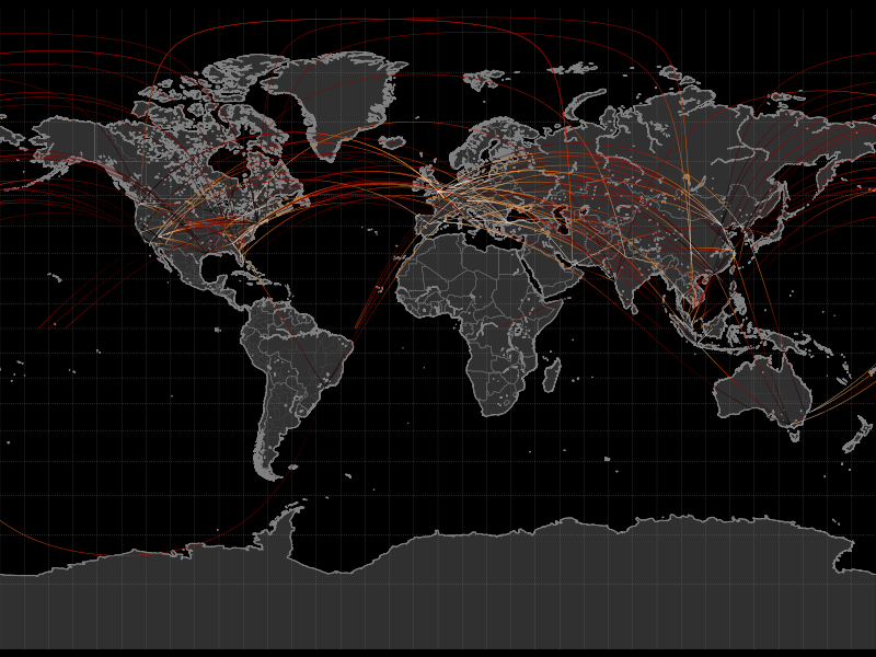
Terrestrial Heat Map (2D Histogram)¶

The simplest display type that Tracktable supports is the 2-dimensional histogram or heatmap. It requires points that contain longitude/latitude coordinates. The points can contain any number of other attributes but they will be ignored.

Run the example as follows:

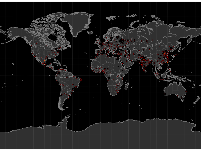
$ python -m "tracktable.examples.heatmap_from_points" TRACKTABLE/examples/data/SampleHeatmapPoints.csv HeatmapExample1.png

Open the resulting image (HeatmapExample1.png) in your favorite image viewer. You will see a map of the Earth with a smattering of red and yellow dots. These are our example points, all generated in the neighborhood of population centers.

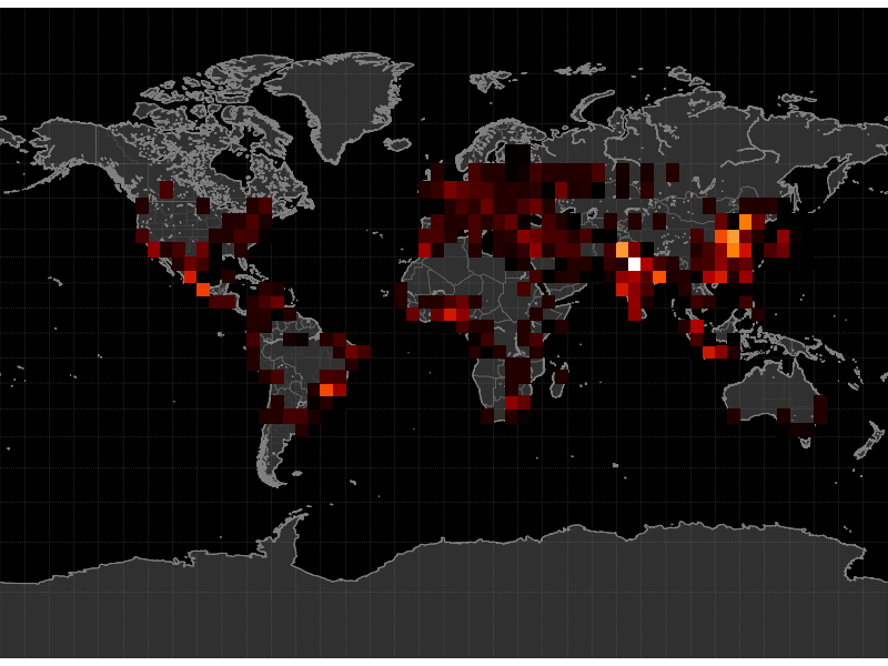
Now it’s time to change things around. Let’s suppose that you want to see larger-area patterns with a coarser distribution. You can change the histogram resolution with the --histogram-bin-size argument:

$ python -m "tracktable.examples.heatmap_from_points" --histogram-bin-size 5 TRACKTABLE/examples/data/SampleHeatmapPoints.csv HeatmapExample2.png

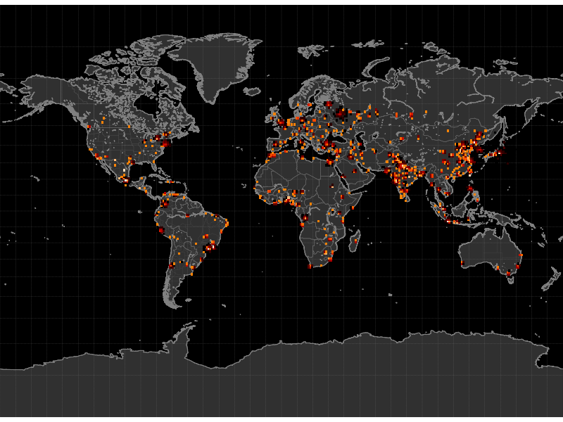
Perhaps when you open up that image you find that the bins are now too large. The earlier size was good but the histogram is too sparse. If you change the color map to use a logarithmic scale instead of a linear one you might get more detail:

$ python -m "tracktable.examples.heatmap_from_points" --scale logarithmic TRACKTABLE/examples/data/SampleHeatmapPoints.csv HeatmapExample3.png

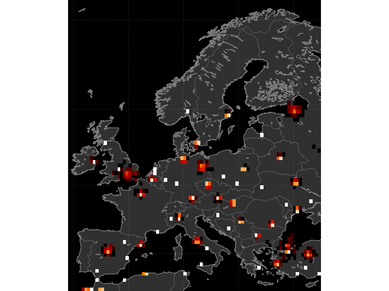
That doesn’t help much. What if we zoom in on Europe and make the bins smaller?

$ python -m "tracktable.examples.heatmap_from_points" --scale logarithmic --map europe --histogram-bin-size 0.5 TRACKTABLE/examples/data/SampleHeatmapPoints.csv HeatmapExample4.png

There are many more options that you can change including map region, point domain (geographic or Cartesian), decoration, colors, image resolution and input configuration. You can get a full list of options with the --help argument:

$ python -m "tracktable.examples.heatmap_from_points" --help

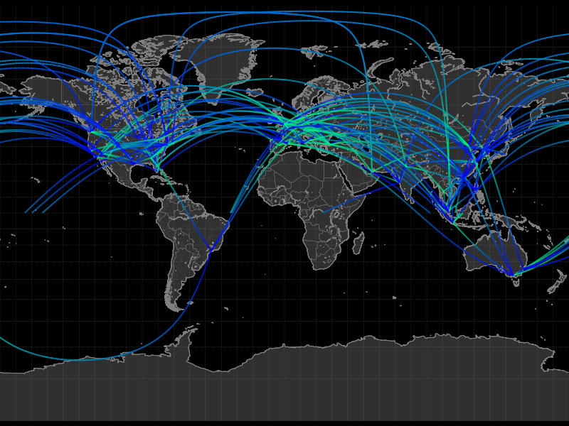
Terrestrial Trajectory Map¶

As soon as we add timestamps to our (longitude, latitude) points we can sensibly assemble sequences of points into trajectories. Trajectories lend themselves to being plotted as lines on a map. That’s our second example. We have provided a sample data set of trajectories between many of the world’s busiest airports for you to use.

$ python -m "tracktable.examples.trajectory_map_from_points"
    TRACKTABLE/examples/data/SampleTrajectories.csv
    TrajectoryMapExample1.png

The trajectories are colored according to the ‘progress’ feature that ranges from 0 at the beginning of a trajectory to 1 at its end. However, the thin lines make them difficult to see with this resolution and color map. Let’s make the lines for the trajectories wider and change the color map.

$ python -m "tracktable.examples.trajectory_map_from_points"
    --trajectory-linewidth 2
    --trajectory-colormap winter
    TRACKTABLE/examples/data/SampleTrajectories.csv
    TrajectoryMapExample2.png

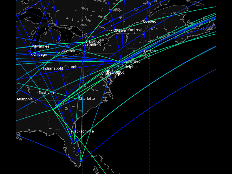
Just for the sake of argument, let’s zoom in on the eastern US. We don’t have a predefined map for that but we can come up with a bounding box. We want the region from (-90, 24) to (-60, 50). Recall that in our longitude-first convention that’s (90W, 24N) to (60W, 50N). While we’re at it, let’s also draw and label every city with a population over half a million people.

$ python TRACKTABLE/examples/trajectory_map_from_points.py
    --trajectory-linewidth 2
    --trajectory-colormap winter
    --map custom
    --map-bbox -90 24 -60 50
    --draw-cities-larger-than 500000
    TRACKTABLE/examples/data/SampleTrajectories.csv
    TrajectoryMapExample3.png

Last and not least, let’s highlight the borders of the US states and Canadian provinces in bright green lines 2 points wide. We’ll also decrease the trajectory width so that the city labels aren’t so overwhelmed. Don’t forget the backslash () in front of the color.

$ python -m "tracktable.examples.trajectory_map_from_points"
    --state-color \#80FF80
    --state-linewidth 2
    --trajectory-linewidth 1
    --trajectory-colormap winter
    --map custom
    --map-bbox -90 24 -60 50
    --draw-cities-larger-than 500000
    TRACKTABLE/examples/data/SampleTrajectories.csv
    TrajectoryMapExample3.png

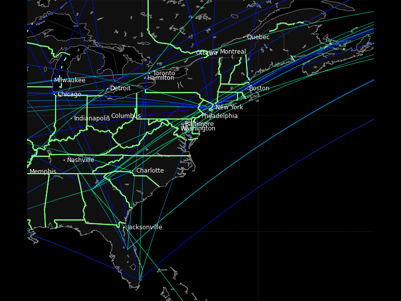
This result is not going to win any beauty contests but you’ve now seen a few more options available to you. Tracktable allows you to change the presence, appearance and style of boundaries for continents, countries and states (US/Canada only at present). You can filter and draw city locations by population (given some minimum threshold) or by ranking. You can change the line style, appearance and color map for the rendered trajectories. All of this is explained in the Using Tracktable With Python and the Reference Documentation.

Cartesian Trajectory Map¶

Since the addition of point domains in Tracktable 0.8 we can use the same rendering code that draws on maps of the world to draw data in flat 2D Cartesian space. You need to specify –domain cartesian2d and –map-bbox x y X Y as follows:

$ python -m "tracktable.examples.trajectory_map_from_points"
     --object-id-column 0
     --timestamp-column 1
     --x-column 2
     --y-column 3
     --delimiter ,
     --map-bbox -100 -100 100 100
     --domain cartesian2d
     TRACKTABLE/examples/data/SamplePointsCartesian.csv
     trajectory_map_cartesian.png

Support for automatically determining the bounding box of the data and adding an appropriate margin is coming soon.

Movies¶

To render a movie, we render short subsets of trajectories over and over. As such we can re-use all of the arguments and algorithms we already have for rendering trajectory maps with just a few additions for movie duration, frames per second, and trajectory length.

Terrestrial Movie¶

We’ll begin with a short movie (10 seconds long, 10 frames per second) where each moving object has a trail showing the last hour of its motion:

$ python -m "tracktable.examples.movie_from_points"
     --trail-duration 3600
     --trajectory-linewidth 2
     --fps 10
     --duration 10
     TRACKTABLE/examples/data/SampleTrajectories.csv
     MovieExample1.mp4

This will encode a movie using vanilla MPEG4 that should be playable by anything less than ten years old. Quicktime Player, iTunes, and Windows Media Player can all handle this. If you don’t already have VLC installed we recommend that as well.

We have two more features to demonstrate here. First, instead of having the trajectory lines be of constant width along their length we can have them taper as they get older. We do this with --trajectory-width taper, trajectory-initial-linewidth and trajectory-final-linewidth. We will also put a dot at the head of each trajectory with --decorate-trajectory-head and trajectory-head-dot-size.

$ python -m "tracktable.examples.movie_from_points"
   --trail-duration 3600
   --trajectory-linewidth taper
   --trajectory-initial-linewidth 3
   --trajectory-final-linewidth 0
   --decorate-trajectory-head
   --trajectory-head-dot-size 3
   --fps 10
   --duration 10
   TRACKTABLE/examples/data/SampleTrajectories.csv MovieExample2.mp4

Too Many Arguments!¶

Response files are used for managing siutations where many command line arguments need to be used. The use of of these files is documented in the user guide (see Using Tracktable With Python).

Cartesian Movie¶

As with geographic data, we can also make movies from data in flat Cartesian space:

$ python -m "tracktable.examples.movie_from_points"

  --domain cartesian2d
  --object-id-column 0
  --timestamp-column 1
  --x-column 2
  --y-column 3
  --delimiter ,
  --map-bbox -100 -100 100 100
  --trajectory-linewidth taper
  --trajectory-initial-linewidth 4
  --trajectory-final-linewidth 1
  TRACKTABLE/examples/data/SamplePointsCartesian.csv
  MovieExample3.mp4

NOTE: The trails won’t appear in the movie until several seconds in. This is not a bug. Recall that trails are colored by their progress from start to finish and the default colormap (“heat”) is black at the beginning. If you would like to see them bright and vivid right from the start, add an argument like --trajectory-colormap prism (or any other Matplotib colormap you like).