Using Tracktable With Python
For this first release we’re going to focus on getting point data into Tracktable and rendered out as a heatmap, trajectory map or movie using the Python interface. We will add more sections to this user guide as we add capability to the toolkit.
Basic Classes
Domains
Tracktable operates on points, timestamps and trajectories. Since points and trajectories are meaningless without a coordinate system, we instantiate points and trajectories from a domain. Each domain provides several different data types and a standard set of units. By design, it is difficult to mix points and trajectories from different domains. While we cannot prevent you entirely from mixing up (for example) kilometers and miles when computing distances, we can at least try to make it difficult.
Tracktable 0.9 includes the following domains:
C++ Namespace |
Python Module |
Description |
|---|---|---|
tracktable::domain::terrestrial |
tracktable.domain.terrestrial |
Points in longitude/latitude space |
tracktable::domain::cartesian2d |
tracktable.domain.cartesian2d |
Points in flat 2D space |
tracktable::doamin::cartesian3d |
tracktable.domain.cartesian3d |
Points in flat 3D space |
Each domain defines several data types:
C++ Class |
Python Class |
Description |
|---|---|---|
base_point_type |
BasePoint |
Bare point - just coordinates. |
trajectory_point_type |
TrajectoryPoint |
Point with coordinates, object ID, timestamp and used-defined properties. |
linestring_type |
LineString |
Vector of un-decorated points (base points). |
trajectory_type |
Trajectory |
Vector of trajectory points. Trajectories have their own user-defined properties. |
base_point_reader_type |
BasePointReader |
Read BasePoints from a delimited text file. |
trajectory_point_reader_type |
TrajectoryPointReader |
Read TrajectoryPoints from a delimited text file. |
box_type |
Box |
Axis-aligned bounding box. |
We provide rendering support for the terrestrial and 2D Cartesian domains via Matplotlib and Basemap. Rendering support for 3D points and trajectories is still an open issue. Given the limited support for 3D data in Matplotlib we may delegate this job to another library. Exactly which library we might choose is open for discussion.
NOTE: In this guide we will assume you are working with TrajectoryPoint data rather than BasePoint data and that you are in the terrestrial domain.
Timestamp
There is a single timestamp class that is common across all point
domains. In C++ this is tracktable::Timestamp, a thinly disguised
boost::posix_time::ptime. In Python this is a timezone-aware
datetime.datetime. As is the case elsewhere in
Tracktable, we convert automatically between the two data types when
Python code calls C++ and vice versa.
The tracktable.core.Timestamp class contains several
convenience methods for manipulating timestamps. A full list is in
the reference documentation. We use the following ones most frequently.
Timestamp.from_any: Try to convert whatever argument we supply into a timestamp. The input can be adict, adatetime, a string in the formatYYYY-MM-DD HH:MM:SSorYYYY-MM-DD HH:MM:SS+ZZ(for a time zone offset from UTC).Timestamp.to_string: Convert a timestamp into its string representation. By default this will produce a string like2014-08-28 13:23:45. Optional arguments to the function will allow us to change the output format and include a timezone indicator.
Base Points
Within a domain, Tracktable uses the BasePoint class to store a bare set of coordinates. These behave like vectors or sequences in that we use square brackets to set and get coordinates:
from tracktable.domain.terrestrial import BasePoint

my_point = BasePoint()
my_point[0] = my_longitude
my_point[1] = my_latitude

longitude = my_point[0]
latitude = my_point[1]
Longitude is always coordinate 0 and latitude is always coordinate 1. We choose this ordering for consistency with the 2D Cartesian domain where the X coordinate is always at position 0 and the Y coordinate is at position 1.
Access a point’s coordinates as if the point were an array using
[]. In Python:
my_point = tracktable.domain.terrestrial.TrajectoryPoint()
longitude = 50
latitude = 40
my_point[0] = longitude
my_point[1] = latitude
my_point.object_id = 'FlightId'
my_point.timestamp = tracktable.core.Timestamp.from_any('2014-04-05 13:25:00')
In C++:
my_point = tracktable::domain::terrestrial::trajectory_point
float longitude = 50, latitude = 40;
my_point[0] = longitude;
my_point[1] = latitude;
my_point.set_object_id("FlightId");
my_point.set_timestamp(tracktable::time_from_string("2014-04-05 13:25:00");
Trajectory Points
The things that make a point part of a trajectory are (1) its coordinates, already covered by BasePoint; (2) an identifier for the moving object, and (3) a timestamp recording when the object was observed. These are the main differences between BasePoint and TrajectoryPoint.
from tracktable.domain.terrestrial import TrajectoryPoint
from tracktable.core import Timestamp

my_point = TrajectoryPoint()
my_point[0] = my_longitude
my_point[1] = my_latitude

my_point.object_id = 'FlyingThing01'
my_point.timestamp = Timestamp.from_any('2015-02-01 12:23:56')
You may want to associate other data with a point as well. For example:
my_point.properties['altitude'] = 13400
my_point.properties['origin'] = 'ORD'
my_point.properties['destination'] = 'LAX'
my_point.properties['departure_time'] = Timestamp.from_any('2015-02-01 18:00:00')
For the most part you can treat the properties array like a Python dict. However, it can only hold values that are of numeric, string or Timestamp type.
Note that the timestamp and object ID properties are specific to trajectory points.
Operations On Points
The module tracktable.core.geomath has most of the
operations we want to perform on two or more points. Here are a few
common ones. These work with both BasePoint and TrajectoryPoint
unless otherwise noted.
distance_between(A, B): Compute distance between A and Bbearing(origin, destination): Compute the bearing from the origin to the destinationspeed_between(here, there): Compute speed between two TrajectoryPointssigned_turn_angle(A, B, C): Angle between vectors AB and BCunsigned_turn_angle(A, B, C): Absolute value of angle between vectors AB and BC
Trajectories
Just as each domain has BasePoint and TrajectoryPoint classes,
we include LineString and Trajectory for ordered sequences of
points.
LineString is analogous to BasePoint in that it has no
decoration at all. It is just a sequence of points. Trajectory
has its own ID (trajectory_id) as well as its own properties
array.
As with point classes above, each domain in Tracktable defines a
trajectory class. A trajectory is just a vector of points with a few
extra properties attached. In C++, a trajectory behaves just like a
std::vector and can be used with the C++ Standard Library as such.
In Python, a trajectory is an iterable just like any other sequence.
Here are examples of creating a trajectory in each language.
C++:
// Assume this array has been populated already
trajectory_point_type my_points[100];


// Initialize with iterators
trajectory_type my_trajectory(my_points, my_points+100);

trajectory_type my_trajectory2;
for (int i = 0; i < 100; ++i) {
   my_trajectory2.push_back(my_points[i]);
}
Python:
# Populate a trajectory from scratch
traj = tracktable.domain.terrestrial.Trajectory()
for point in mypoints:
    traj.append(mypoint)
Tracktable expects that all points in a given trajectory will have the same object ID. Timestamps must not decrease from one point to the next.
There are several free functions defined on trajectories that do useful things. We expect that the following will be used most often:
point_at_time(trajectory: Trajectory, when: Timestamp): Given a timestamp, interpolate between points on the trajectory to find the point at exactly the specified time. Timestamps before the beginning or after the end of the trajectory will return the start and end points, respectively. Tracktable will try to interpolate all properties that are defined on the trajectory points.subset_in_window(trajectory: Trajectory, start, end: Timestamp): Given a start and end timestamp, extract the subset of the trajectory between those two times. The start and end points will be at exactly the start and end times you specify. These will be interpolated if there are no points in the trajectory at precisely the right time. Points in between the start and end times will be copied from the trajectory without modification.recompute_speed,recompute_heading: Compute new values for thespeedandheadingnumeric properties at each point given the position and timestamp attributes. These are convenient if our original data set lacks speed/heading information or if the original values are corrupt.
Input
There are three ways to get point data into Tracktable in version 0.9.9. We can instantiate and populate TrajectoryPoint objects by hand, load points from a delimited text file, or create them algorithmically.
If we choose to create points algorithmically we will need to supply (at a minimum) coordinates, a timestamp and an ID.
Loading Points from Delimited Text
Tracktable has a flexible point reader for delimited text files. The bare class is the templated PointReader in the IO directory. Each point domain provides two versions of it, one for loading base points (coordinates only) and one for loading trajectory points.
Python Example
from tracktable.domain.terrestrial import TrajectoryPointReader


     with open('point_data.csv', 'rb') as infile:
         reader = TrajectoryPointReader()
         reader.input = infile
         reader.delimiter = ','

         # Columns 0 and 1 are the object ID and timestamp
         reader.object_id_column = 0
         reader.timestamp_bolumn = 1

         # Columns 2 and 3 are the longitude and
         # latitude (coordinates 0 and 1)
         reader.coordinate_column[0] = 2
         reader.coordinate_column[1] = 3

         # Column 4 is the altitude
         reader.numeric_fields["altitude"] = 4

         for point in reader:
              # Do whatever you want with the points here
Point Sources
There are algorithmic point generators in the
tracktable.source.path_point_source module that are suitable for
trajectory-building. The ones most likely to be useful are
GreatCircleTrajectoryPointSource
and LinearTrajectoryPointSource.
Give them start and end points, start and end times, a number of
points to generate and an object ID and you should be ready to go.
Assembling Points into Trajectories
Creating trajectories from a set of points is simple conceptually but logistically annoying when we write the code ourselves. The overall idea is as follows:
Group points together by object ID and increasing timestamp.
For each object ID, connect one point to the next to form trajectories.
Break the sequence to create a new trajectory whenever it doesn’t make sense to connect two neighboring points.
This is common enough that Tracktable includes a filter
(tracktable.source.trajectory.AssembleTrajectoryFromPoints)
to perform the assembly starting from a Python iterable of points
sorted by non-decreasing timestamp. We can specify two parameters to
control part 3 (when to start a new trajectory):
separation_time: Adatetime.timedeltaspecifying the longest permissible gap between points in the same trajectory. Any gap longer than this will start a new trajectory.separation_distance: Maximum permissible distance (in kilometers) between two points in the same trajectory. Any gap longer than this will start a new trajectory.
We can also specify a minimum_length. Trajectories with fewer than
this many points will be silently discarded.
Example
trajectory_builder = AssembleTrajectoryFromPoints()
trajectory_builder.input = point_reader

trajectory_builder.separation_time = datetime.timedelta(minutes=30)
trajectory_builder.separation_distance = 100
trajectory_builder.minimum_length = 10

for traj in trajectory_builder.trajectories():
     # process trajectories here
Annotations
Once we have points or trajectories in memory we may want to annotate them with derived quantities for analysis or rendering. For example, we might want to color an airplane’s trajectory using its climb rate to indicate takeoff, landing, ascent and descent. we might want to use acceleration, deceleration and rates of turning to help classify moving objects.
The module tracktable.feature.annotations contains functions to do
this. Every feature defined in that package has two functions
associated with it: a calculator and an accessor. The calculator
computes the values for a feature and stores them in the trajectory.
The accessor takes an already-annotated trajectory and returns a
1-dimensional array containing the values of the already-computed
feature. This allows us to attach as many annotations to a
trajectory as we like and then select which one to use (and how) at
render time.
Todo
Code example for annotations
Rendering
Now we come to the fun part: making images and movies from data.
Tracktable 0.9.0 supports three kinds of visualization: a heatmap (2D histogram), a trajectory map (lines/curves drawn on the map) and a trajectory movie. We render heatmaps directly from points. Trajectory maps and movies require assembled trajectories.
In all cases we render points into a 2D projection. Here in the user’s guide we will discuss rendering onto a map projection. The procedure for rendering points in Cartesian space is very similar and will be documented Real Soon Now.
We use the Basemap toolkit for the map projection and Matplotlib for the actual rendering.
Setting Up a Map
The easiest way to create and decorate a map is with the
tracktable.render.mapmaker.mapmaker() function. It can
create maps of common (named) areas of the world, regions surrounding
airports, and user-specified regions. Here’s an example that will
create a map of Australia with coastlines and longitude/latitude
graticules rendered every 2 degrees.
from tracktable.render.mapmaker import mapmaker
from matplotlib import pyplot

f = pyplot.figure(size=(8, 6), dpi=100)

(mymap, initial_artists) = mapmaker('australia',
                                    draw_coastlines=True,
                                    draw_countries=False,
                                    draw_states=False,
                                    draw_lonlat=True,
                                    lonlat_spacing=2,
                                    lonlat_linewidth=0.5)
We always return two values from Mapmaker. The first is the
mpl_toolkits.basemap.Basemap instance that will convert
points between world coordinates (longitude/latitude) and map
coordinates. The second is a list of Matplotlib artists that define all the decorations added to
the map.
There are several predefined map areas. Their names can be retrieved
by calling tracktable.render.maps.available_maps(). If you
would like to have a region included please send us its name and
longitude/latitude bounding box. We will add it to the next release.
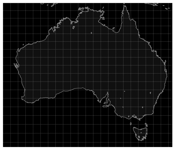
This map of Australia was generated by passing the map name
australia to Mapmaker.
This next example will render a 200x200 km area around Boston’s Logan Airport (BOS). Coastlines will be drawn with an extra-thick (2-point-wide) red line. US state borders will be drawn in blue. Land will be filled in using solid white. We use high-resolution borders since we’re zoomed in fairly far.:
from tracktable.render.mapmaker import mapmaker
from matplotlib import pyplot

f = pyplot.figure(size=(8, 6), dpi=100)
(mymap, initial_artists) = mapmaker('airport:BOS',
                                    border_resolution='h',
                                    draw_coastlines=True,
                                    draw_states=True,
                                    land_color='white',
                                    coastline_color='red',
                                    coastline_linewidth=2,
                                    country_color='blue')
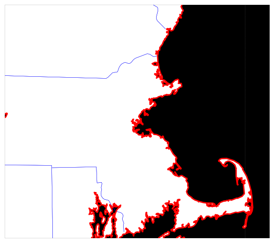
This map of the area around Boston’s Logan Airport was generated by
passing the map name airport:BOS to Mapmaker.
Note
The underlying maps.map_for_airport() function allows
you to change the size of the displayed area from 200x200 km
to anything you want. We will expose this parameter via
Mapmaker in a future release. In the meantime, if you need
that level of control we suggest using map_name =
'custom' and map_bbox to get the area you need.
If we want a map that does not correspond to any of the predefined ones then we can use the ‘custom’ map type. This example will create a map of Japan and the Korean Peninsula with all cities labeled whose population is larger than 2 million.
from tracktable.render.mapmaker import mapmaker
from matplotlib import pyplot

f = pyplot.figure(size=(8, 6), dpi=100)

# Bounding box is [ longitude_min, latitude_min,
#                   longitude_max, latitude_max ]
(mymap, initial_artists) = mapmaker(
           'custom',
           map_bbox = [ 123.5, 23.5, 148, 48 ],
           draw_cities_larger_than=2000000
      )
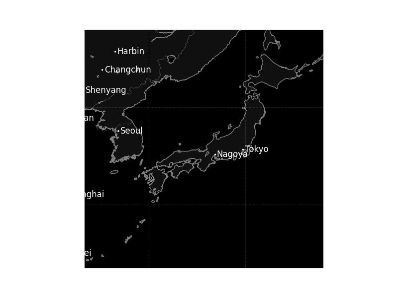
This map was generated by passing the map name custom and a
longitude/latitude bounding box to Mapmaker.
Note
To define a map area that crosses the discontinuity at longitude +/- 180 degrees, use coordinates that wrap around beyond 180. The bounding boxes (-200, 0, -160, 40) and (160, 0, 200, 40) both define a region that extends from 0 to 40 degrees latitude and 20 degrees to either side of 180 degrees longitude.
Todo
We haven’t described how to set up a map projection for the Cartesian domain.
Rendering Onto the Map
Since Tracktable uses Matplotlib as its
underlying renderer you can immediately render almost anything you
want on top of a map. Remember, however, that Matplotlib does not
know about the map projection. In order to draw things that will be
properly registered onto the map you need to use the
Basemap instance that we
got earlier when we set up our map using Mapmaker. By calling the map
instance as if it were a function you can convert coordinates from
world space (longitude/latitude) to axis space (arbitrary coordinates
established by Matplotlib).
There are many ways to draw things like contours, points, curves, glyphs and text directly onto the map. Please refer to the example gallery for demonstrations. Tracktable provides code to render two of the most common use cases for trajectory data: heatmaps (2D histograms) and trajectory maps.
Heat Maps
A heat map (Wikipedia page) is a two-dimensional histogram – that is, a density plot. We use heat maps to illustrate the density of points that compose a set of trajectories. We are typically looking for areas of high traffic and areas of coverage.
This release of Tracktable supports heat maps rendered on top of
geographic maps using the
tracktable.render.histogram2d.geographic function. You
must call it with at least two arguments – a Basemap instance and an iterable of points.
Other optional arguments will let you control the histogram bin size,
color map and where on the map the heatmap is rendered.
We include a start-to-finish example of how to load points and render
a heat map in the heatmap_from_csv.py script in the
tracktable/examples/ subdirectory of our Python code. This
example has its own page in the
documentation.
Note
The histogram2d.geographic() heat map
generator only traverses its input data once to keep memory
requirements low. You can safely use it with point sets too
large to load into memory at once.
Trajectory Maps
A trajectory map is an ordinary map with one or more trajectories drawn on it. We may want to decorate a trajectory with any of the following:
Colors defined as a function of some quantity computed for the trajectory such as speed, turn rate or altitude
Variable line widths (such as a trajectory that is broad at its head and narrow at its tail)
A dot of some color and size at the head of the trajectory to mark the object’s actual position
A label at the head of the trajectory to display an object ID
All of this is packaged into the function draw_traffic in the
tracktable.render.paths module.
Note
The argument names for that function are slightly
misleading. Pay careful attention to the documentation for
that function. Specifically, the arguments
trajectory_linewidth_generator and
trajectory_scalar_generator seem to indicate by their
names that you must compute the linewidths and scalars at
render time. This is fine for single images. For movies,
we find it more useful to compute as much as we can before
rendering and then pass an accessor function in as the
generator.
Like heat maps, trajectory maps have
their own example script trajectory_map_from_csv.py in the
tracktable/examples directory. This script has its own page in the documentation.
Making Movies
To a first approximation, making a movie is the same as making a single image many, many times. The part that takes some care is minimizing the number of times we perform expensive operations such as loading data and configuring/decorating a map.
Our approach looks like this:
all_data = load_data()
figure = setup_matplotlib_figure()
setup_map_projection(figure)
movie_writer = setup_movie_writer()

with movie_writer.saving(figure, 'movie_filename.mp4'):
    for frame_num in xrange(num_frames):
        frame_data = render_frame(frame_num, all_data)
        movie_writer.grab_frame()
        cleanup_frame(frame_data)
The setup phase is exactly the same as it would be if we were
rendering a single image. The conceptual differences are in
render_frame(), which must take into account which frame it’s
drawing, and cleanup_frame(), which restores the drawing area to
its beginning-of-frame state. We adopt the convention that
render_frame() shall return a list of all Matplotlib artists that
were added to the figure while rendering the current frame. That way
we can clean up by removing each artist after the frame has been saved
by a call to movie_writer.grab_frame().
Although Matplotlib supports several different animation back ends including live on-screen animation, Mencoder, FFMPEG, ImageMagick, Tracktable 0.9.0 only supports the FFMPEG back end. There are two reasons. First, FFMPEG is available for nearly all platforms and is quite capable. By supporting it before any others we can help as many users as possible render movies as quickly as possible. Second, FFMPEG has a few extra capabilities that make it well suited to rendering movies in parallel.
Please refer to the files example_movie_rendering.py,
movie_from_csv.py and parallel_movie_from_csv.py in the
directory tracktable/Python/tracktable/examples for an
illustration of how to render a movie. More thorough documentation
will follow soon.
Command Line
Tracktable’s various rendering facilities have a lot of options. Python makes it easy for us to expose these as command-line options that can be passed to scripts. However, that just pushes the problem out one level: now the user has to remember the values for all of those options, or else write shell scripts that call Python scripts in order to keep track of what parameters were used where.
We introduce two facilities to help tame this morass:
Argument Groups: An argument group is a set of command-line arguments that all pertain to a single capability. For example, the argument group for trajectory assembly has entries for the maximum separation distance, maximum separation time and minimum length as described above in Assembling Points into Trajectories.
Response Files: A response file is a way to package up arbitrarily many command-line arguments in a file and pass them to a script all at once. It is independent of which script is being run. Since a response file is just text it is easy to place under version control. We provide a slightly modified version of the standard Python
argparsemodule that includes support for response files containing comments and response files that load other response files.
Argument Groups
The point of an argument group is to save us from having to cut and paste the same potentially-lengthy list of arguments and their respective handlers into each new script we write. When we render a movie of data over time, for example, we will always need several pieces of information including resolution, frame rate, and the duration of our movie.
Since we’re human we are guaranteed to forget an argument here, spell one differently there, and before long we have a dozen scripts that all take completely different command-line arguments. Bundling arguments in an easy-to-reuse fashion makes it easy for us to use the same ones consistently.
We derive another benefit at the same time. By abstracting away a set of arguments into a semi-opaque module, we can add capability to (for example) the mapmaker without having to change our movie-making script. Once the argument group for the mapmaker is updated, any script that uses the mapmaker’s argument group will automatically gain access to the new capability.
There are three parts to using argument groups. First they must be
created and registered. Second, they are applied when we create an
argument parser for a script. Finally, once command-line arguments
have been parsed, we (as the programmers) can extract values for each
argument group that you used. All of these functions are in the
tracktable.script_helpers.argument_groups.utilities module.
Creating an Argument Group
We create an argument group first by declaring it with
create_argument_group()
and then populating it with calls to
add_argument(). Here is an example from the movie_rendering group:
create_argument_group("movie_rendering",
                      title="Movie Parameters",
                      description="Movie-specific parameters such as frame rate, encoder options, title and metadata")

add_argument("movie_rendering", [ "--duration" ],
             type=int,
             default=60,
             help="How many seconds long the movie should be")

add_argument("movie_rendering", [ "--fps" ],
             type=int,
             default=30,
             help="Movie frame rate in frames/second")

add_argument("movie_rendering", [ "--encoder-args" ],
             default="-c:v mpeg4 -q:v 5",
             help="Extra args to pass to the encoder (pass in as a single string)")
All of Tracktable’s standard argument groups are in files in the
Python/tracktable/script_helpers/argument_groups directory. Look
at __init__.py in that directory for an example of how to add one
to the registry. You can register your own groups anywhere in your
code that you choose.
Applying Argument Groups
We use argument groups by applying their arguments to an
already-instantiated argument parser. That can be an instance of the
standard argparse.ArgumentParser or our customized version
tracktable.script_helpers.argparse.ArgumentParser. Here
is an example:
from tracktable.script_helpers import argparse, argument_groups

parser = argparse.ArgumentParser()
argument_groups.use_argument_group("delimited_text_point_reader", parser)
argument_groups.use_argument_group("trajectory_assembly", parser)
argument_groups.use_argument_group("trajectory_rendering", parser)
argument_groups.use_argument_group("mapmaker", parser)
We can interleave calls to use_argument_group()
freely with calls to other functions defined on
ArgumentParser.
We recommend reading the code for
use_argument_group()
if you need to do especially complex things with argparse such
as mutually exclusive sets of options.
Using Parsed Argument Values
After we call parser.parse_args() we are left with a Namespace
object containing all the values for our command-line options, both
user-supplied and default. We use the extract_arguments()
function to retrieve sets of arguments that we configured using
use_argument_group().
Our practice is to define handler functions that take every argument
in a group so that we can write code like the following:
def setup_trajectory_source(point_source, args):
    trajectory_args = argument_groups.extract_arguments("trajectory_assembly", args)
    source = example_trajectory_builder.configure_trajectory_builder(
        **trajectory_args
       )
    source.input = point_source

    return source.trajectories()
Since we are not required to refer to the individual arguments directly the user can take advantage of new capabilities added to the underlying modules whether or not we know about them when we write our script.
Todo
Add tracktable.script_helpers.argument_groups to the documentation
Response Files
Todo
Document response files in full
Once we start calling scripts with more than 3 or 4 options it becomes
difficult to keep track of all the arguments and difficult to edit the
command line. We address this with response files, textual listings
of command-line options and their values that we can pass to scripts.
The standard Python argparse module has limited support for
response files. We expand upon it with our own extended argparse.
Fuller documentation is coming soon. This should be enough to get you started:
$ cd tracktable/Python/tracktable/examples
$ python heatmap_from_csv.py --write-response-file > heatmap_response_file.txt
Now open up heatmap_response_file.txt in your favorite editor.
Lines that begin with # are comments. Uncomment any arguments you
please and add or change values for them. After you save the file,
run the script as follows:
$ python heatmap_from_csv.py @heatmap_response_file.txt
That will tell the script to read arguments from
heatmap_response_file.txt as well as from the command line.
You can freely mix response files and standard arguments on a single command line. You can also use multiple response files. The following command line would be perfectly valid:
$ python make_movie.py @hd_movie_params.txt @my_favorite_map.txt movie_outfile.mkv
Have fun!