Demo 3: Travel Prediction Using Alignment
This notebook describes how to use well-aligned historical trajectories to predict qualities about an observed trajectory’s travel. Namely, in this notebook we predict the origin/destination location of an observed trajectory and the location of an observed trajectory in a specified amount of time.
In [1]:
from tracktable.applications.prediction import *
from tracktable_data.data import retrieve
import os.path
Load in the Data
We read in the file containing historical trajectories and store all relevant information in a dictionary. In our case, the dataset is a ~500 trajectory subset from one day of flight data over the US airspace. While using the full day of flight data (or even more data) would yield better predictions, we use a subset to cut down on the time required to process historical trajectories.
In [2]:
historical_data_file = retrieve(filename='prediction_historical_trajectories.traj')
In [3]:
prediction_dictionary = process_historical_trajectories(historical_data_file,  # file containing historical trajectories
                                               separation_time=20, # minutes
                                               separation_distance=100, # km
                                               minimum_length=20, # km
                                               minimum_total_distance=200, # km
                                               only_commercial=True # relevant for flight data
                                               )
INFO:tracktable.applications.prediction:Begin constructing feature vectors from all points
[2025-06-11 13:01:22.081598] [0x00000001f1aadf00] [info] Read a total of 479 trajectories.
100%|██████████████████████████████████████████████████████████████████████████████████████████████████████████████████████████████████████████████| 479/479 [00:00<00:00, 2219.73it/s]
INFO:tracktable.applications.prediction:Begin constructing RTree
100%|██████████████████████████████████████████████████████████████████████████████████████████████████████████████████████████████████████| 64356/64356 [00:00<00:00, 10348436.90it/s]
INFO:tracktable.applications.prediction:Begin creating segment representation for all trajectories
100%|██████████████████████████████████████████████████████████████████████████████████████████████████████████████████████████████████████████████| 479/479 [00:00<00:00, 3594.98it/s]
Read in the file containing the observed trajectories into a list
In [4]:
observed_data_file = retrieve(filename='prediction_observed_trajectories.traj')

observed_trajectories = TrajectoryReader()
observed_trajectories.input = open(observed_data_file, 'r')
observed_trajectories = list(observed_trajectories)
[2025-06-11 13:01:24.041080] [0x00000001f1aadf00] [info] Read a total of 14 trajectories.
Visualize the Dataset
The number of trajectories in the historical data is…
In [5]:
len(prediction_dictionary['trajectories'])
Out[5]:
479
An image of the historical data is shown below. We use a static image instead of an interactive map to lighten the load on the browser. If you would rather have the interactive map, uncomment and run the line of code in the cell below.
In [ ]:
# render_trajectories(prediction_dictionary['trajs'], backend='folium', tiles='CartoDBPositron')

The number of observed trajectories is….
In [6]:
len(observed_trajectories)
Out[6]:
14
Let’s draw them on a map. We note that the observed trajectories are just short fragments that include no information about their final destinations.
In [7]:
render_trajectories(observed_trajectories, backend='folium', tiles='CartoDBPositron')
Out[7]:
Prediction
Step 1: Choose an observed trajectory for prediction
Choose an observed trajectory from the list.
In [8]:
observed_trajectory = observed_trajectories[0]
Choose how many sample points to represent the observed trajectory with. The sample points (samples) are evenly spaced points along the observed trajectory. The first and last sample points in the list are the end points of the observed trajectory. The fewer the sample points, the less detailed the representation of the observed trajectory. For example, if 2 sample points are used, the observed trajectory is represented as a line segment. Change this number from 2 to 4 to see the difference in representation.
In [9]:
sampled_trajectory = sample_trajectory(observed_trajectory, 2)
In [10]:
render_trajectories([observed_trajectory, sampled_trajectory], line_color=['blue', 'red'], backend='folium', tiles='CartoDBPositron', show_points=True)
Out[10]:
Step 2: Alignment
Alignment is the central, driving algorithm of prediction. It finds well-aligned historical trajectories that are similar in shape and relative location to an observed trajectory. These well-aligned historical trajectories can be used to fill in unknown qualities about an object’s motion (observed trajectory). Two applications of alignment are origin/destination prediction and time-based location prediction. We show those here.
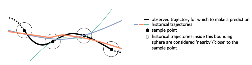
A historical trajectory is well-aligned with an observed trajectory if for each sample point of the observed trajectory, the distance to the historical trajectory is less than the neighborhood distance (radius of circles in image above). The orange historical trajectory is well aligned with the black historical trajectory above. The align function returns a dictionary which maps each historical trajectory to the number of sample points it is close to. We then filter this dictionary to contain only the trajectories that are close to all of the sample points.
In [11]:
neighborhood_distance = 10
In [12]:
well_aligned_trajectories = find_well_aligned_trajectories(sampled_trajectory, prediction_dictionary, neighborhood_distance)
100%|████████████████████████████████████████████████████████████████████████████████████████████████████████████████████████████████████████████████████| 2/2 [00:00<00:00, 96.16it/s]
Step 3: Direction check
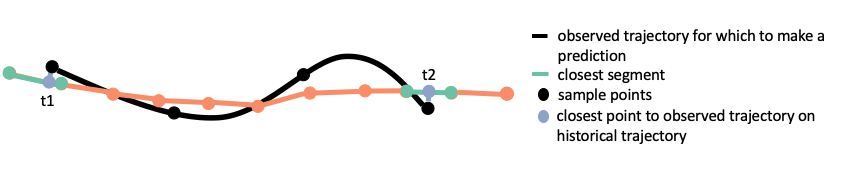
To determine if a historical trajectory is going in the same direction as an observed trajectory, first, represent the historical trajectory using segments. Find the closest segment of the historical trajectory to the first and last points in time of the observed trajectory. Interpolate along these two segments to find the closest point in space on the historical trajectory to the first and last point of the observed trajectory. Let t1 be the time of the point on the historical trajectory closest to the first point of the observed trajectory in space. Let t2 be the time of the point on the historical trajectory closest to the last point of the observed trajectory in space. If t2 - t1 > 0 then the historical trajectory and the observed trajectory are going in the same direction.
In [13]:
same_direction = find_same_direction_trajectories(sampled_trajectory, well_aligned_trajectories, prediction_dictionary)
100%|█████████████████████████████████████████████████████████████████████████████████████████████████████████████████████████████████████████████████| 62/62 [00:00<00:00, 259.15it/s]
Step 4: Assign a weight to each trajectory
The weight assigned to a trajectory is a function of the distance of the sample point that is farthest away from that trajectory. Here, a trajectory’s weight is this distance scaled linearly by the neighborhood distance (1 is the weight if the trajectory and sample point overlap, 0 is the weight if the distance from the trajectory to the sample point is neighborhood distance).
In [14]:
weight_function = lambda d: 1 - d / neighborhood_distance
In [15]:
weights = find_weights_trajectories(sampled_trajectory, same_direction, prediction_dictionary, weight_function)
Optionally, trajectories can be grouped by origin/destination pair during this step. Weights are then assigned to each origin/destination pair. This is not shown above, but is used for origin/destination prediction.
Make Predictions
Use the two prediction functions to link all of these steps together.
Origin/Destination prediction
We can make a prediction about the observed trajectory’s orign and destination. On this list of predictions, a higher weight corresponds to a more likely prediction. Optionally, set the neighborhood distance (how close well-aligned historical trajectories must be to the sample points of the observed trajectory).
In [16]:
results = predict_origin_destination(observed_trajectory,
                                     prediction_dictionary,
                                     samples=4,
                                     neighbor_distance=10 #km
                                    )
100%|███████████████████████████████████████████████████████████████████████████████████████████████████████████████████████████████████████████████████| 4/4 [00:00<00:00, 142.49it/s]
100%|█████████████████████████████████████████████████████████████████████████████████████████████████████████████████████████████████████████████████| 60/60 [00:00<00:00, 267.69it/s]
INFO:tracktable.applications.prediction:List of possible origin destinations with weights:
INFO:tracktable.applications.prediction:Orig    Dest    Weight
INFO:tracktable.applications.prediction:KDEN    KLAS    0.45
INFO:tracktable.applications.prediction:KDEN    KASE    0.20
INFO:tracktable.applications.prediction:KORD    KSFO    0.07
INFO:tracktable.applications.prediction:KDEN    KGJT    0.07
INFO:tracktable.applications.prediction:KDEN    KSNA    0.04
INFO:tracktable.applications.prediction:KDEN    KSFO    0.04
INFO:tracktable.applications.prediction:CYYZ    KLAX    0.04
INFO:tracktable.applications.prediction:KMKE    KLAS    0.04
INFO:tracktable.applications.prediction:KMDW    KLAS    0.03
INFO:tracktable.applications.prediction:KDEN    KLAX    0.01
INFO:tracktable.applications.prediction:10 possible prediction(s)
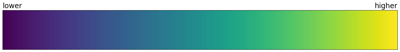
We can also visualize the trajectories leading to this prediction. The observed trajectory is displayed in red. The trajectories from the historical dataset that passed nearby the observed trajectory are displayed in colors corresponding to their position on the prediction list, as shown below:
In [17]:
gradient = np.linspace(0, 1, 256)
gradient = np.vstack((gradient, gradient))

plt.figure(figsize=(20, 2))
ax = plt.axes()
ax.get_xticklabels()
ax.imshow(gradient, aspect='auto', cmap=plt.get_cmap('viridis'))
ax.tick_params(labelbottom=False, labelleft=False, bottom=False,
                left=False)
plt.title('lower', fontsize=20, loc='left')
plt.title('higher', fontsize=20, loc='right')

plt.show()
In [18]:
# origin_destination_render(observed_trajectory, results, prediction_dictionary)

# pick one trajectory to render for each OD pair
possibilities = []
for prediction in results['predictions']:
    trajectories = results['OD_pairs_to_trajs'][prediction]
    possibilities.append(prediction_dictionary['trajectories']
                            [prediction_dictionary['id_to_index'][trajectories[0]]])

# render trajectories in different colors
cmap = matplotlib.cm.get_cmap('viridis')
colors = []
for x in range(0, len(possibilities)):
    rgb = cmap(x * (1 / len(possibilities)))[:3]
    colors.append(matplotlib.colors.to_hex(rgb))
# reverse so that more likely predictions have lighter colors
colors.reverse()

# make the sub trajectory red
possibilities.append(observed_trajectory)
colors.append('red')
map_canvas = render_trajectories(possibilities, line_color=colors, show=True, save=False,
                    backend='folium', tiles='CartoDBPositron', filename='pred_results.html',
                    attr='.', crs='EPSG3857')
/var/folders/dt/9gwr5c3j3nn6jqfwgz9whk5h000bm6/T/ipykernel_87821/122597687.py:11: MatplotlibDeprecationWarning: The get_cmap function was deprecated in Matplotlib 3.7 and will be removed in 3.11. Use ``matplotlib.colormaps[name]`` or ``matplotlib.colormaps.get_cmap()`` or ``pyplot.get_cmap()`` instead.
  cmap = matplotlib.cm.get_cmap('viridis')
Time-based location prediction
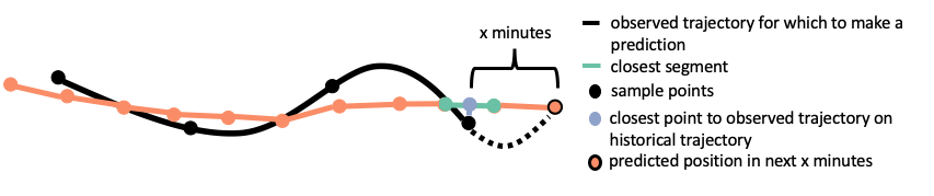
Time-based location prediction is done in a similar way to the direction check. First, represent a well-aligned historical trajectory using segments. Find the closest segment of the historical trajectory to the last point in time of the observed trajectory. Interpolate along this segment to find the closest point in space on the historical trajectory to the last point of the observed trajectory. Find the point on the historical trajectory that is x minutes from this point. This is the predicted location in x minutes and the portion of the historical trajectory between these two points is its predicted path.
We can make a prediction about where the observed object will be in a given number of minutes (in this case 30). Optionally, set the neighborhood distance (how close well-aligned historical trajectories must be to the sample points of the observed trajectory).
In [19]:
points, paths, weights = predict_location(observed_trajectory, prediction_dictionary, minutes=30, samples=4, neighbor_distance=10)
100%|███████████████████████████████████████████████████████████████████████████████████████████████████████████████████████████████████████████████████| 4/4 [00:00<00:00, 141.93it/s]
100%|█████████████████████████████████████████████████████████████████████████████████████████████████████████████████████████████████████████████████| 60/60 [00:00<00:00, 267.07it/s]
Again, we can visualize the historical trajectories leading to this prediction. The trajecories from the historical dataset that passed nearby the observed trajectory are displayed in grey. They represent the possible future paths of the observed trajectory. The white dots represent the possible locations the observed trajectory will be in the specified amount of time. The color of the heatmap corresponds to the likelihood the observed object will be in a given region in the specified amount of time, as shown below:
In [20]:
gradient = np.linspace(0, 1, 256)
gradient = np.vstack((gradient, gradient))

plt.figure(figsize=(20, 2))
ax = plt.axes()
ax.get_xticklabels()
ax.imshow(gradient, aspect='auto', cmap=plt.get_cmap('viridis'))
ax.tick_params(labelbottom=False, labelleft=False, bottom=False,
                left=False)
plt.title('lower', fontsize=20, loc='left')
plt.title('higher', fontsize=20, loc='right')

plt.show()

In [21]:
def heat_map_helper(points, weights):
    """Creates the approriate point formatting to use a heatmap

    Arguments:
        points: list of points to format
        weights: the weights those points received in the prediction algorithm

    Returns: a list of properly formatted points to feed into a heatmap
    """

    return [[points[key][1], points[key][0], weights[key]]
            for key in points.keys()]
In [22]:
# pos_heatmap(points, paths, weights, observed_trajectory)

# create the heat map
heat_map = folium.Map(tiles='CartoDBPositron', zoom_start=4)

# lat, long, weight of points to render
display_points = heat_map_helper(points, weights)
to_render = list(paths.values())

# group all trajectories (including observed trajectory) in one list for rendering
to_render.append(observed_trajectory)
colors = ['grey'] * len(paths)
colors.append('red')
gradient = matplotlib_cmap_to_dict('viridis')
heat_map = render_trajectories(to_render, map_canvas=heat_map, backend='folium',
                                line_color=colors, linewidth=1.0,
                                tiles='CartoDBPositron', attr='.', crs='EPSG3857')
HeatMap(display_points, gradient=gradient).add_to(heat_map)

heat_map
Out[22]:
Create a small relevant data file.
First, make a list of relevant trajectories. This can be done in two ways for predictions:
In [23]:
relevant_trajectories = find_relevant_trajectories_origin_destination(results, prediction_dictionary)
In [24]:
relevant_trajectories = find_relevant_trajectories_location(points, prediction_dictionary)
Then, write these trajectories to a .traj file.
In [25]:
write_trajectories('subset.traj', relevant_trajectories)
Now, instead of loading from a large historical data file, you can load only the trajectories used in the prediction.