Demo 2: Detecting “Boxes”

For each trajectory, we will use Tracktable to generate a score for “boxiness”, where 0 indicates no “boxiness” and 1 indicates that a trajectory moves an equal distance in only four directions, and that those four directions are at 90-degree intervals. In some datasets, such as maritime data, this behavior is especially anomalous, and this will allow us to examine the highest-scoring trajectories for unusual behavior.

Algorithm Details

For a given trajectory, we first examine a histogram of the headings for every linear segment of the trajectory, binned to the nearest degree (i.e. bins for 0, 1, …, and 359 degrees). We will deviate from traditional binning: instead of adding a value of one for each segment with a given heading, we add the length of the segment. This is done to allow for nonuniform sampling along our trajectory. Once all segment lengths have been added to the respective heading bins, we normalize by dividing by the length of the trajectory. If there is a box present in our data, we expect this histogram to have peaks at four bins spaced in 90-degree intervals. For this reason, we multiply to form quartets that represent a score for each of these possible rotated boxes. That is, we multiply the bin values at 0, 90, 180 and 270 degrees to get a score for the 0-degree quartet. We would expect this number to be higher if there is a box at this 0-90-180-270 orientation, and lower (or zero) if not. The 1-degree quartet is found by multiplying the bin values at 1, 91, 181, and 271 degrees, and so on, until we have quartets 0 through 89. Roughly speaking, each quartet represents a score proportional to the likelihood that the trajectory creates a box at a given orientation. If we sum these values, then a uniform headings histogram would yield a maximum boxiness score, which is not desirable. So instead, we use a window (by default 5 degrees wide) centered at the maximum quartet value to score our trajectory for “boxiness”. Lastly, we normalize by the largest possible quartet, (0.25)^4, so that a perfect box will have a “boxiness” score of 1. Note: We use this method because trajectories creating perfect boxes are guaranteed to have high “boxiness” scores. However, it’s important to note that it is possible for other trajectories to score high despite not having boxes. For instance, the two trajectories below will both have a perfect boxiness score of 1:

1. A trajectory that travels due north for 10km, then due east for 10km, then due south for 10km, then due west for 10km, forming a perfect square.

2. A trajectory that travels due south for 10km, then due east for 5km, then due west for 10km, then due east for 5km, then due north for 10km, making a 90 degree angular pattern but not a box.

from tracktable.render.render_trajectories import render_trajectories
from tracktable.algorithms.boxiness import calculate_boxiness, sort_by_boxiness
import tracktable.examples.tutorials.tutorial_helper as tutorial

Import Trajectories

We will use some sample maritime data for this demo obtained from the Bureau of Ocean Energy Management.\(^1\)

trajectories = tutorial.get_trajectory_list('boxiness')

Loading Trajectories: 125 trajectory [00:00, 1423.74 trajectory/s]

[2025-06-11 12:55:23.842917] [0x00000001f1aadf00] [info]    Read a total of 125 trajectories.

This dataset contains 125 trajectories. Our goal is to identify any trajectories that form unusually boxy patterns, and to do so more efficiently that by visual inspection of all 125 trajectories.

Option 1: Calculate boxiness for a single trajectory.

trajectory = trajectories[7]

Let’s see what this trajectory looks like.

render_trajectories(trajectory)

Make this Notebook Trusted to load map: File -> Trust Notebook

The calculate_boxiness function will score the trajectory for boxiness as described in “Algorithm Details” above, and has the following parameters:

• The window parameter allows us to change the width of the window (centered at the peak quartet) over which we sum to calculate boxiness. By default, window is five degrees.

Once boxiness has been calulcated, it is stored in trajectory.properties['boxiness'].

calculate_boxiness(trajectory, window=7)

How boxy is the trajectory? A score of 1 corresponds to a perfect square, and a score of 0 means no “boxiness” was detected.

Note: Depending on the dataset, scores much less than one may still indicate interesting “boxiness” behavior, and so the threshold for “interesting” should be application dependent.

trajectory.properties['boxiness']

2.300405528284749e-08

Option 2: Calculate boxiness for a list of trajectories.

We can do this calculation on a list of trajectories as well, and each trajectory’s “boxiness” score will be stored in trajectory.properties['boxiness'].

calculate_boxiness(trajectories)

Let’s see a histogram of the boxiness scores of our trajectories:

import matplotlib.pyplot as plt

# make a new matplotlib figure
fig = plt.figure(figsize=(20,10))

# label the axes
plt.xlabel('boxiness scores')
plt.ylabel('number of trajectories')

# make a histogram of the boxiness scores
plt.hist(x=[trajectory.properties['boxiness'] for trajectory in trajectories], bins=100);

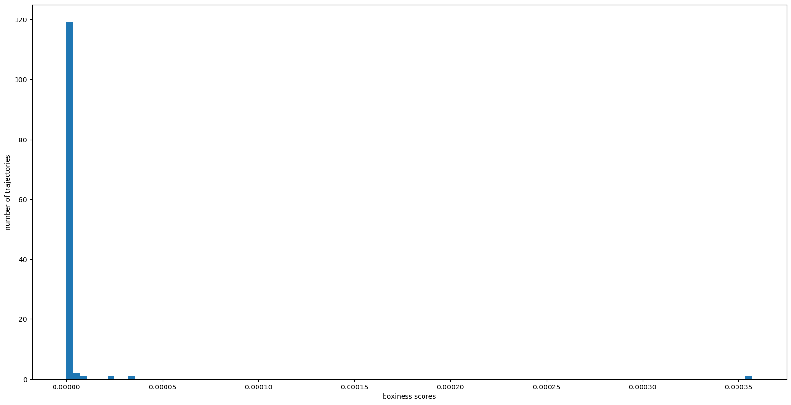
It’s looks like we have one outlier trajectory with much higher boxiness than the rest. Our third option, shown below, will sort our trajectories by boxiness so that we can easily identify the boxiest trajectories.

Option 3: Calculate boxiness and sort trajectories by boxiness.

Note: If boxiness has already been calculated and stored as a property, set calculate_boxiness to False to improve computation time.

trajectories_sorted_by_boxiness = sort_by_boxiness(trajectories,
                                                   calculate_boxiness=False)

Visualize Boxiest Trajectories

What does our boxiest trajectory look like?

render_trajectories(trajectories_sorted_by_boxiness[0], show_points=True)

Make this Notebook Trusted to load map: File -> Trust Notebook

\(^1\) Bureau of Ocean Energy Management (BOEM) and National Oceanic and Atmospheric Administration (NOAA). MarineCadastre.gov. AIS Data for 2020. Retrieved February 2021 from marinecadastre.gov/data. Data is for June 4-6, 2020 martime traffic near Virginia Beach.